Rows in Excel provide a structured way for all the users to organize and reference data in an Excel worksheet.
In this article, you will learn every detail about rows in Excel.
After reading this blog post, you will learn how to:
– Select rows
– Insert, delete, hide, unhide, group, and ungroup rows
– Move rows
– Modify row height
– Refer to rows in formulas
– Count rows in a range
– Limit rows in a sheet
Note: We have used Excel for Microsoft 365 to prepare this tutorial.
⏷What Is Excel Row?
⏷Selecting Rows
⏷How to Insert Rows
⏷How to Delete Rows
⏷Hide and Unhide Rows
⏷How to Group Rows
⏷How to Ungroup Rows
⏷How to Move Rows
⏷Modifying Row Height
⏷Referring to a Row in Formula
⏷Getting Number of Rows in a Range
⏷Limiting the Number of Rows in Sheet
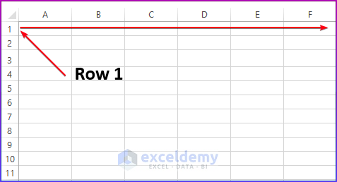
What Is Excel Row?
In Microsoft Excel, a row is a horizontal arrangement of cells that runs the worksheet from left to right. Each row is identified by the unique number on its left side from where it started.
Horizontal rows are numbered with numeric values such as 1, 2, 3, etc. usually displayed on the left side of the spreadsheet. A total 1,048,576 numbers of rows are stored in a spreadsheet.
The first row is commonly used for column headings or titles, and it is often referred to as the Header Row.
The final row in Excel is labeled as 1,048,576, and this number is unchangeable; additional rows cannot be added to a sheet. To incorporate more data, the solution is to insert a new worksheet, which will also consist of the same fixed number of rows.
To navigate the last row in Excel, click the Control + Down Arrow keys.
How to Select a Row in Excel?
In this part, we will discuss how to select rows in Excel using various methods with a keyboard shortcut.
1. Selecting Entire Row
To select an entire row in the worksheet, select a cell (in this case, B10) of the target row and then press the Shift + Spacebar shortcut.
Now, you can see that the 10th row has been selected in the following GIF.
2. Selecting Adjacent Rows
To select adjacent rows in the worksheet, press the Shift + Spacebar keys ⇒ press the Down Arrow key holding the Shift + Spacebar keys.
Finally, you will see that rows have been highlighted from the 11th row to the 14th row.
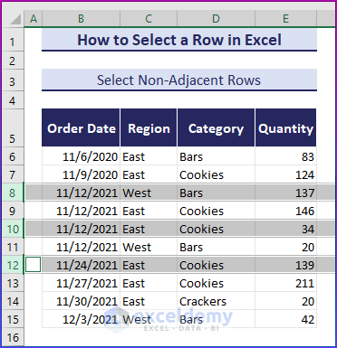
3. Selecting Non-Adjacent Rows
You can simply select non-adjacent rows by holding the Ctrl key and clicking on the row numbers.
To select the 8th row, click the row number with your mouse.

After that, hold down the Ctrl key ⇒ to select adjacent rows (in this case, the 10th and 12th rows) using your mouse.
4. Selecting Multiple Rows Using the Name Box
Apart from the common methods of selecting rows in Excel, there’s another useful trick using the Name Box.
- Click on the Name box to enable it.
- Write the reference for the row range you wish to choose. For example, use “8:12” in the Name box to select rows 8 through 12.
- Press Enter.
- You can see all the steps and the output in the following GIF.
5. Selecting All Rows Below
In Excel, you can also use the Ctrl + Shift + Down Arrow shortcut to select all rows that are below a certain position.
Follow the detailed instructions below:
- Choose the first cell in the row from where you want to start the selection.
- To expand the selection to as many columns as required, hold down the Shift key and press the Right Arrow key.
- Once you have selected all the required columns, release the Shift key.
- It’s time to select every row below a specific position. Press the Ctrl+Shift+Down arrow keys simultaneously.
Excel will choose all the rows automatically below, starting from the first point you choose and continuing to the very last row of data in your dataset.
6. Select Rows with a Certain Value in Column
You can use the Filter tool to select all rows that have a certain value in a particular column. To filter and choose the appropriate rows, follow the following actions:
Follow the Steps Below:
Select any cell in the dataset ⇒ Click on the Filter Tool in the Data tab.
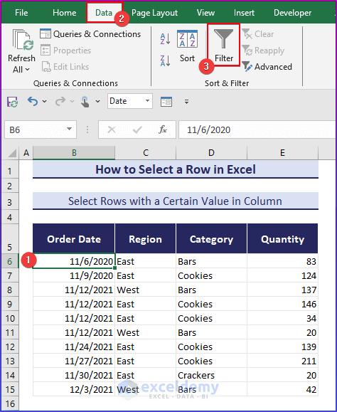
You can see the Filter drop-down in each column header.
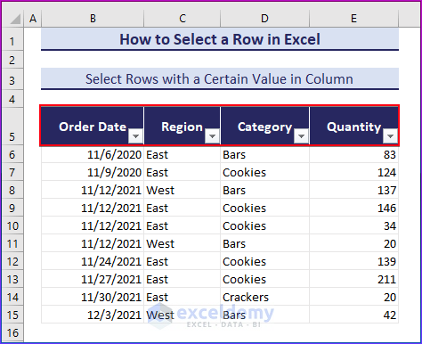
Click the Filter arrow in the column that contains the specific value you wish to filter.
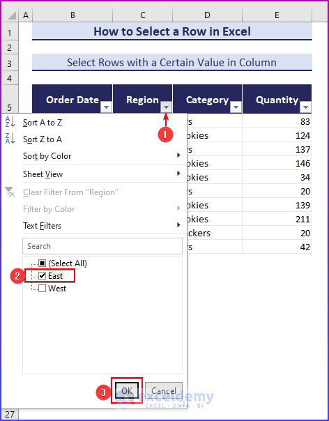
Then select the desired value or values from the drop-down menu. Excel will display only the rows that contain the selected value after filtering the data.
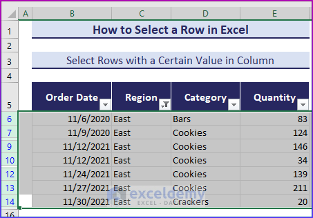
After applying the filter, you can select the filtered rows using the Mouse.
How to Insert Rows in Excel?
In this part, we will guide you on how to insert rows in Excel using the Insert Option, Keyboard shortcut, Name Box, and Copy and Paste method.
1. Insert Multiple Rows in Excel Using the Insert Option
In this part, we will show how to insert multiple rows from the Context Menu and Top Ribbon.
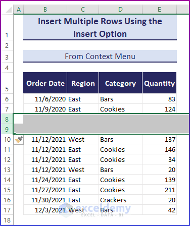
1.1 From Context Menu
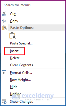
To insert rows in a worksheet, select rows using the mouse and right-click on the selected rows.
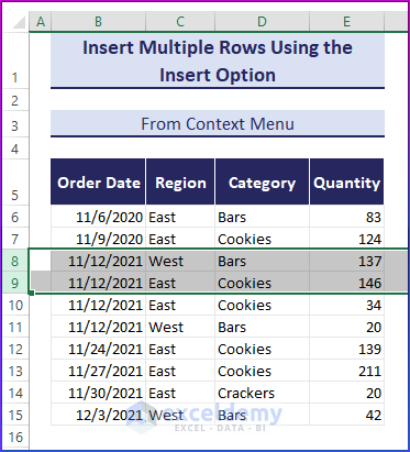
Click on the Insert Option from the menu.
You can see that new rows have been added.
Read More: How to Create Rows within a Cell in Excel
1.2 From Top Ribbon
To insert rows in a worksheet, select rows using the mouse ⇒ go to the Home tab ⇒ click the icon of the Insert command from the Cells group ⇒ click on the Insert Sheet Rows option.
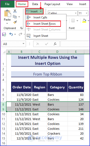
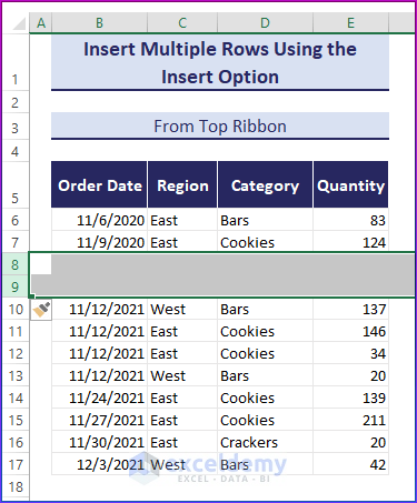
You can see that new rows have been added.
2. Insert Multiple Rows Using a Keyboard Shortcut
To insert multiple rows, select any cell where you want to insert your new row.
- Apply the shortcut method and press Shift + Spacebar to select the entire row
- Press the Shift + Down arrow keys to select the number of rows you want to insert.
- Press the Ctrl + Shift + Plus sign keys to insert your new rows.
- In the following GIF, you can see rows have been inserted.
3. Insert Multiple Rows Using the Name Box
To insert multiple rows using the Name Box, select the cell above where you want to insert rows. For example, we will select the B9 cell.
- Write the range 9:12 (according to your preference) and press Enter.
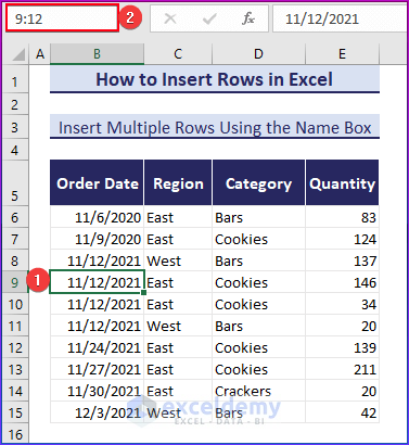
- All the rows have been selected from 9th to 12th.
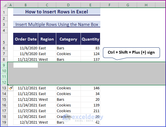
- Now, press the Ctrl + Shift + Plus (+) sign to insert rows into your worksheet.
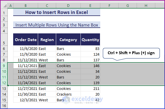
- Finally, you can see all the rows have been inserted from 9th to 12th.
Read More: How to Insert Row in Excel
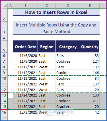
4. Insert Multiple Rows Using the Copy and Paste Method
To insert multiple rows with cell data, select the rows you want to insert.
Copy all the selected rows by pressing Ctrl + C.
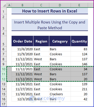
Select the same number of rows using the mouse where you want to insert your new rows.
Right-click on the selected rows, and then a menu will appear. Click on the Insert Copied Cells option to insert your copied rows in your spreadsheet.
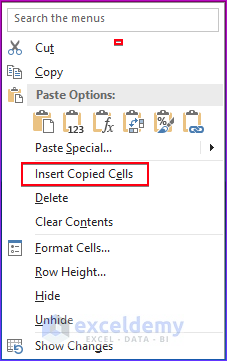
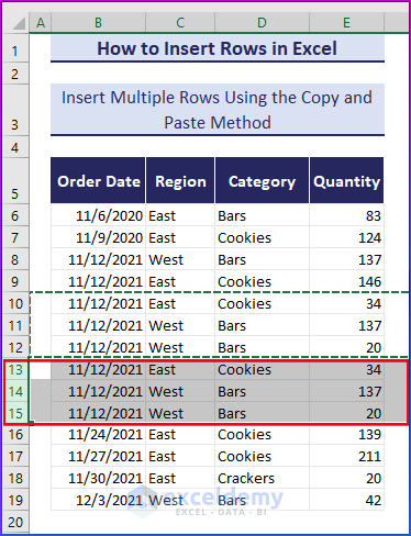
Finally, you can see all the copied rows (from the 10th to the 12th) have been inserted in the 13th, 14th, and 15th positions.
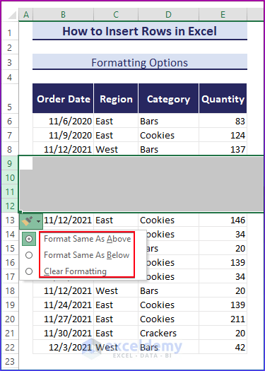
Formatting Options Appearing After Inserting New Row in Excel
After inserting new rows, you will see a Format button appear. After clicking on that, you will get three options:
- Format Same as Above: Apply the same formatting (such as font style, cell borders, and background color) to the added row to match the format of the rows above.
- Format Same as Below: Apply formatting (such as font style, cell borders, and background color) to the inserted row to align with the format of the rows below.
- Clear Formatting: Removes all formatting.
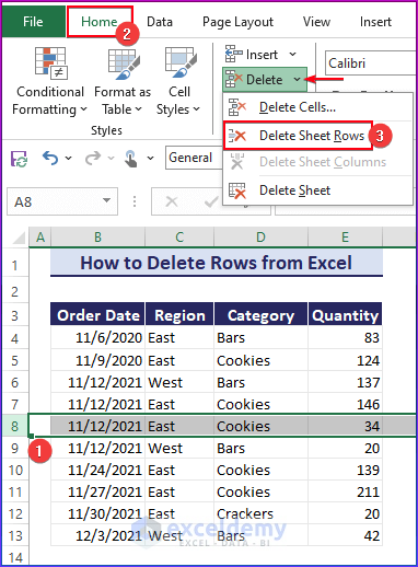
How to Delete Rows from Excel?
To delete an entire row, select row 8 ⇒ Home tab ⇒ click on Delete Sheet Rows from the Delete drop-down menu.
Read More: How to Delete Rows in Excel
How to Hide and Unhide a Row in Excel?
First, click on the row number ⇒ drag down the cursor to select the rows you want to hide.
To hide rows from 9-11, select rows 9,10,11⇒ Then go to the Home tab ⇒ click the icon of the Format command from the Cells group ⇒ click on the Hide & Unhide option ⇒ select the Hide Rows option.
You can see all the rows have been hidden.
You can unhide all the rows using the same procedure, and then click on the Unhide Rows option.
Now, all the rows are visible again
Read More: How to Hide Rows in Excel
How to Group Rows in Excel?
We can group rows in Excel in two easy ways: Manually and Automatically.
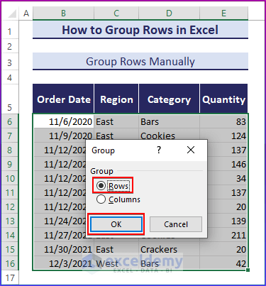
1. Group Rows Manually
To group rows manually, select data range B6:E16 ⇒ Go to the Data tab ⇒ click on Group from the Outline section.
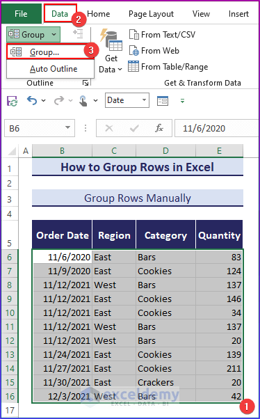
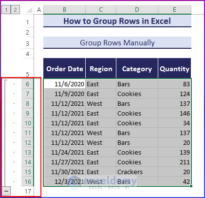
A pop-up window named Groupe will appear before you. Select Rows from there.
You can see that all the selected rows have been grouped.
2. Group Rows Using Auto Outline Command
To group rows automatically, go to the Data tab ⇒ select Auto Outline from the Group drop-down.
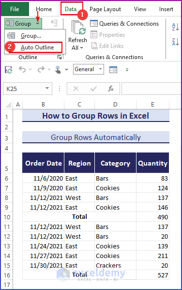
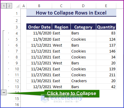
Finally, you can see the group has been created automatically.
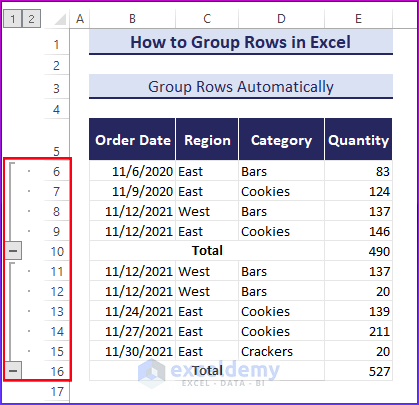
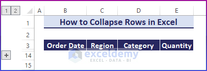
To collapse rows in an Excel worksheet, just click the – (Minus) button, as shown in the following image.
The collapsed row is now visible in the following image.
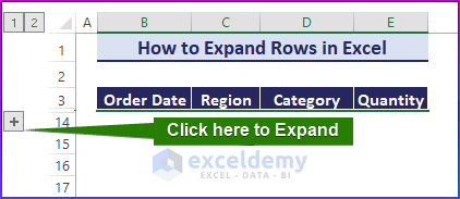
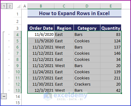
To expand rows in your Excel worksheet, click on the + (Plus) icon as shown in the following image.
You will now see the extended rows in the following image.
Read More: How to Expand and Collapse Rows in Excel
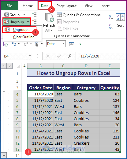
How to Ungroup Rows in Excel?
To ungroup rows, Select data range B6:E16 ⇒ Go to the Data tab ⇒ select the Ungroup option from the Outline section.
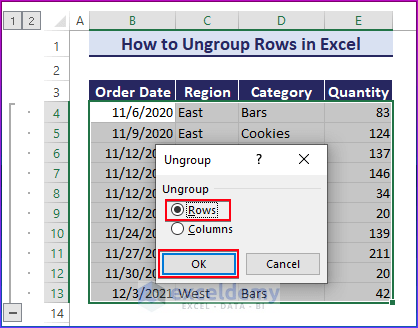
A pop-up window named Groupe will appear before you. Select Rows from there.
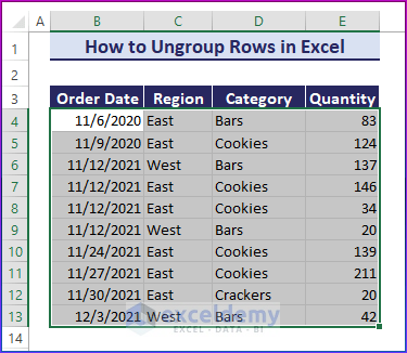
Finally, you can see the group has been removed from rows.
How to Move Rows in Excel?
The Excel Cut command is a valuable tool for relocating rows. The selected row can be inserted into either an empty row or another already occupied row, replacing the row.
To move a row,
- Select the row (e.g. row 8) ⇒ select the Scissor-shaped icon (Cut Option) under the Home tab
- Then, select the target row (e.g row 14 or any other row where you want to insert the cut row ⇒ select the Paste under the Home
Now, you can see that row 8 has been moved to a new position ( row 14).
Read More: How to Move Rows in Excel
How to Modify Row Height in Excel?
In this section, we will show how to modify and autofit row height and set a custom height.
1. Modify Row Height by Dragging the Mouse
To modify row height, keep the cursor on row 5 ⇒ Adjust the row height by clicking and dragging the mouse upwards to increase it or downwards to decrease ⇒ Simply release the mouse button, and the selected row’s height will be changed.
Read More: Row Height Excel (All Things You Need to Know)
2. AutoFit Row Height
You can see that the rows are not adjusted here. So, we will adjust the row height with the text.
To do this, select the rows ⇒ Then go to the Home tab ⇒ click the icon of the Format command from the Cells group ⇒ click on the AutoFit Row Height option.
You can see the process and the output in the following GIF.
3. Set Custom Row Height
To set custom height according to your preference, Then go to the Home tab ⇒ click the icon of the Format command from the Cells group ⇒ click on the Row Height option.
Here, we will keep the row height at 20. You can see the changes in the following GIF.
How to Refer to Rows in Excel Formulas?
To refer to a row, you can use its number. Now, we will refer to row 9, then we will use the following address in the SUM function.
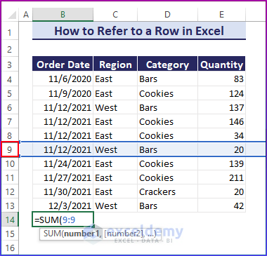
Now, you can see that it will refer to row 9 in the following image.
How to Get the Number of Rows in a Range of Cells?
We will use the ROW function to get the number of rows in a range. The ROWS function returns the number of rows in a reference or an array. It doesn’t require any arguments, and you simply provide a reference or array as its input.
Here’s the basic syntax:
=ROWS(reference)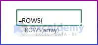
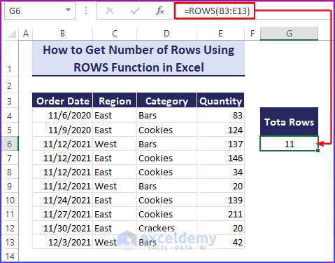
For example: we will select range B3:E13 from our dataset to count the number of rows.
- Select cell G6.
- Apply the following formula in cell G6.
=ROWS(B3:E13)Now, you can get the number of rows in the following image.
How to Limit the Number of Rows?
Sometimes, you may need to limit the number of rows to avoid showing all the Excel data to others. Follow the below steps accordingly.
- To keep the last row visible, click the row number below it.
- Press the Down Arrow key while holding down Ctrl + Shift This will select all the remaining rows from the selected row in the worksheet
- Now, go to the Home tab ⇒ click on the arrow from the Format option under the Cells group ⇒select Hide & Unhide ⇒ click on Hide Rows from the drop-down menu.
This will hide every other row in your worksheet below the final row you have selected to remain visible.
Download Practice Workbook
In this article, we have discussed how to select, insert, group, modify, move, delete, hide, and unhide rows in the Excel workbook. You can learn how to count the number of rows in a range, and I have explained everything, from how to expand, collapse, and ungroup rows in Excel. We have also discussed the common scenario of navigating, limiting, and referring rows in Excel. Please share your thoughts with us in the comment box.
Rows in Excel: Knowledge Hub
- How to Create Collapsible Rows in Excel
- How to Color Alternate Rows in Excel
- How to Lock Rows in Excel
- How to Expand or Collapse Rows with Plus Sign in Excel
- How to Resize All Rows in Excel
- How to Number Rows in Excel
- How to Get Excel Row Number
<< Go Back to Learn Excel