When working with huge datasets in Excel, it is common to wish to lock some rows or columns. So we can see their contents while navigating to another part of the worksheet. This article explains how to lock rows in Excel so that they remain visible while moving to another section of the worksheet.
How to Lock Rows in Excel: 6 Easy and Simple Ways
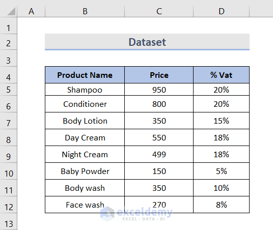
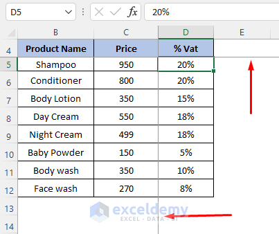
The dataset we are using to lock rows contains some products and their prices and percentage of value-added tax (VAT).
1. Lock Rows Using Freeze Panes Feature
It only takes a few clicks to lock rows in Excel. Let’s go through the following steps to see how this feature works to lock rows in Excel.
1.1. Lock Top Rows
Assuming we are working with a dataset that has headers at the top row and a dataset that traverses many rows when we look down, the headers/names would disappear. In such cases, it’s smart to lock the header line so that these are dependably noticeable to the user. Here are the steps to lock the top row.
Steps:
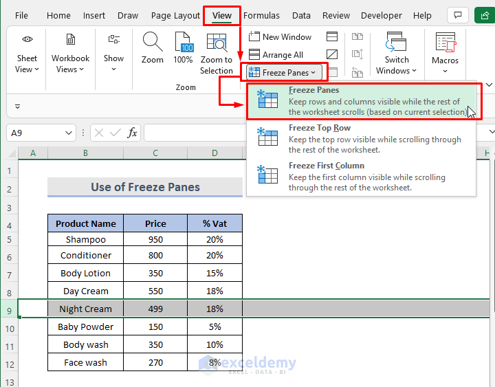
- Firstly, go to the View tab on the ribbon.
- Select the Freeze Panes and choose Freeze Top Row from the drop-down menu.
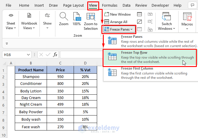
- This will lock the first row of your worksheet, ensuring that it remains visible when you browse through the remainder of it.
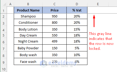
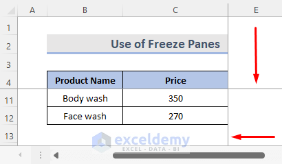
- Now, if we scroll down, we can determine that the top row is frozen.
1.2. Lock Several Rows
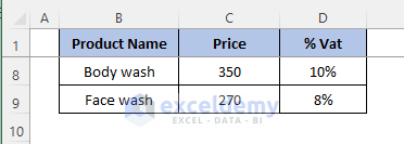
We may wish to keep specific rows in our spreadsheet visible all of the time. We can scroll over our content and still see the frozen rows.
Steps:
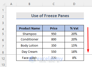
- Select the row below, the rows we want to freeze. In our example, we want to freeze rows 1 to 8. So, we’ll select row 9.
- Click the View tab on the ribbon.
- In the Freeze Panes drop-down menu, choose the Freeze Panes option.
- The rows will lock in place, as demonstrated by the gray line. We can look down the worksheet while scrolling to see the frozen rows at the top.
Read More: How to Create Rows within a Cell in Excel
2. Excel Magic Freeze Button to Freeze Rows
The Magic Freeze button can be added to the Quick Access Toolbar to freeze rows, columns, or cells with a single click.
Steps:
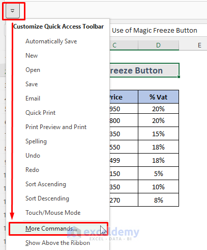
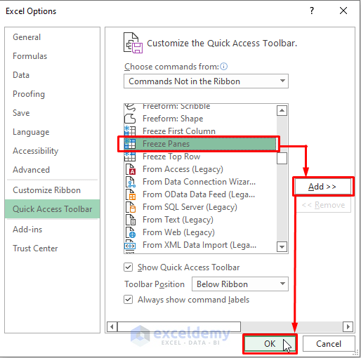
- Go to the drop-down arrow from the top of the Excel file.
- Click on More Commands from the drop-down.
- From the Quick Access Toolbar, choose Commands Not in the Ribbon.
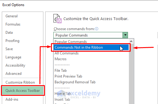
- Scroll down and find the Freeze Panes option then select it.
- At last, click on Add and then OK.
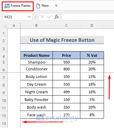
- Freeze Panes are shown above on the Name Box. We can now access the freeze panes option quickly.
- After clicking on the Freeze Panes button, the columns and rows will be frozen at the same time.
3. Lock Rows Using the Split Option in Excel
Splitting a worksheet region into many pieces is another approach to freeze cells in Excel. Freeze Panes keep specific rows or columns displayed while scrolling through the spreadsheet. Splitting Panes divides the Excel window into two or four sections, each of which can be scrolled independently. The cells in the other areas remain fixed when we scroll within one region.
Steps:
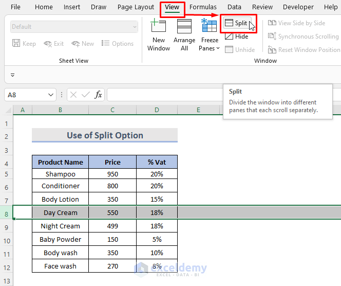
- First, select the row below that we want to split.
- Click the Split button on the View tab.
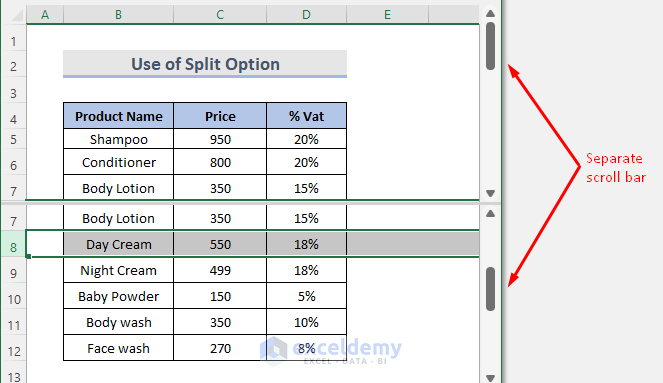
- Now, we can see two separate scroll bars. To reverse a split, click the Split button once again.
4. Use VBA Code to Freeze Rows
We can also use the VBA code to lock the rows.
Steps:
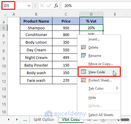
- Firstly, we have to select any cell below where we want to lock the rows and columns at the same time.
- Right-click on the spreadsheet and select View Code.
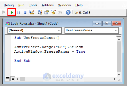
- Then, a VBA Module window appears where we will write the code.
VBA Code:
Sub UseFreezePanes()
ActiveSheet.Range("D5").Select
ActiveWindow.FreezePanes = True
End Sub- Copy and paste the above code. Click on Run or use the keyboard shortcut (F5) to execute the macro code.
- Finally, all the rows and columns are locked in the worksheet.
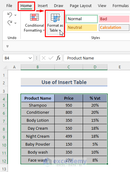
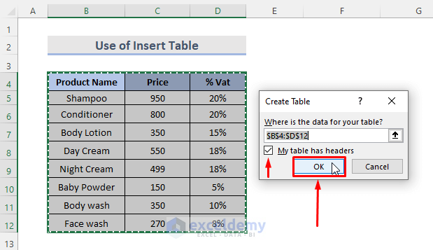
5. Insert Excel Table to Lock Top Row
Assuming that you’d like the header column to consistently remain fixed at the top while you look down, convert a range to a fully functional table.
Steps:
- First, select the whole table. Next, go to the Home tab > Format as Table.
- Now, the table is selected and a pop-up window appears.
- The checkmark on the My Table has headers.
- Then, click on the OK button.
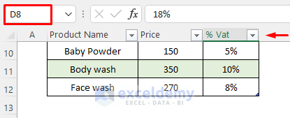
- This will make your table fully functional.
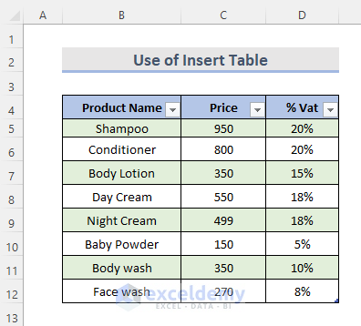
- If we scroll down, we can see our headers are shown on top.
6. Lock Both Rows and Columns in Excel
In most circumstances, we have the header and labels in rows as well as columns. In such circumstances, freezing both rows and columns makes sense.
Steps:
- Choose a cell that is just below the rows and close to the column we wish to freeze. For example, if we want to freeze rows 1 to 4 and columns A, B, C. Then, we will select cell D5.
- After that, go to the View tab.
- Click on the Freeze Panes drop-down.
- Select the Freeze Panes option from the drop-down.
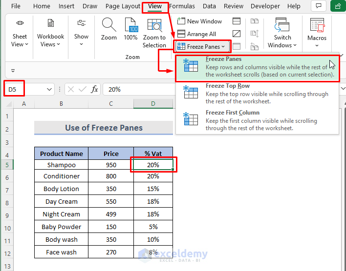
- The columns to the left of the selected cell and the rows above the selected cell will be frozen. Two gray lines appear, one just next to the frozen columns and the other directly below the frozen rows.
Freeze Panes aren’t Operating Properly to Lock Rows in Excel
If the Freeze Panes button in our worksheet is disabled, it’s most likely for one of the following reasons:
- We are in cell editing mode, which allows us to do things like entering a formula or changing data in a cell. Press the Enter or Esc key to leave cell editing mode.
- Our spreadsheet is protected. Please unprotect the worksheet first, then freeze the rows or columns.
Notes
You can freeze only the top row and the first left column. You can’t freeze the third column and nothing else around it.
Download Practice Workbook
You can download the workbook and practice with them.
Conclusion
By following these methods, you can easily lock rows in your workbook. All those methods are simple, fast, and reliable. Hope this will help you! If you have any questions, suggestions, or feedback please let us know in the comment section.
Related Articles
- How to Resize All Rows in Excel
- How to Number Rows in Excel
- How to Create Collapsible Rows in Excel
- How to Expand and Collapse Rows in Excel
- How to Expand or Collapse Rows with Plus Sign in Excel
- How to Copy Every Nth Row in Excel
- How to Color Alternate Rows in Excel
<< Go Back to Rows in Excel | Learn Excel

