An Excel drop down list is a feature that allows users to select an element from a list of options. It is used to create a list of homogeneous elements and make it easy to pick one from a large amount of data. It is frequently used in data entry forms, user interface, data analysis and filtration, etc.
In this free Excel tutorial, we will explain the processes of creating, editing, removing, filtering, etc of an Excel drop down list.
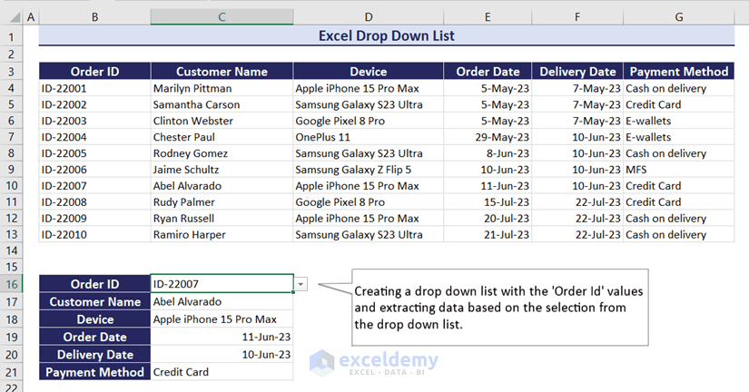
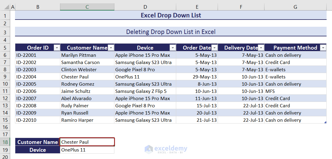
Here, I have a dataset of online shopping information in the ‘Order ID’, ‘Customer Name’, ‘Device’, ‘Order Date’, ‘Delivery date’, and ‘Payment Method’ columns. I have created a drop down list with the values from ‘Order ID’ and extracted related information with the selected ID from the drop down list.
In this article, you will learn how to create a drop down list-
-from a range of cell
-from a table
-from name range
-from another worksheet
-from another workbook
You will also learn creating a dependent drop down list, searchable drop down list, dynamic drop down list, editable drop down list, etc. We will also discuss how you can protect & delete an Excel drop down list and how to solve different issues related to the drop down.
⏷What Is a Drop Down List in Excel?
⏷How to Create a Drop Down List in Excel?
⏵1. Drop Down List from a Range of Cells
⏵2. Drop Down List from Table
⏵3. Drop Down List with Named Range
⏵4. Drop Down List with Color
⏵5. Drop Down List with Unique Values
⏵6. Drop Down List Based on Data from Another Sheet
⏵7. Drop Down List Based on Data from Another Workbook
⏵8. Creating a Dependent Drop Down List
⏵9. Making a Searchable Drop Down List
⏵10. Creating a Dynamic Drop Down List
⏵11. Creating a Searchable, Dynamic, and Multi-dependent Drop Down List
⏵12. Making a Drop Down List with Custom Message
⏵13. Creating an Editable Drop Down List with Error Alert Message
⏷How to Add or Remove Items from Excel Drop Down List?
⏷How to Protect Drop Down List in Excel?
⏷How to Delete Drop Down List in Excel?
⏷How to Filter Drop Down List & Extract Data Based on Selection in Excel?
⏷How to Solve Issues with Excel Drop Down List?
What Is a Drop Down List in Excel?
A drop down list in Excel is a list of predefined values that allows you to select an element from that list. We often create a drop down list of homogeneous elements. A drop down list makes it easy to pick an element from a list of homogeneous options from a large set of data.
How to Create a Drop Down List in Excel?
Using a range of cells, a table, or a named range are the three most common ways of creating a drop down list in Excel. Creating a drop down list from data in another worksheet or workbook is also possible. A drop down list can be dependent, independent, searchable, editable too.
1. Creating a Drop Down List from a Range of Cells
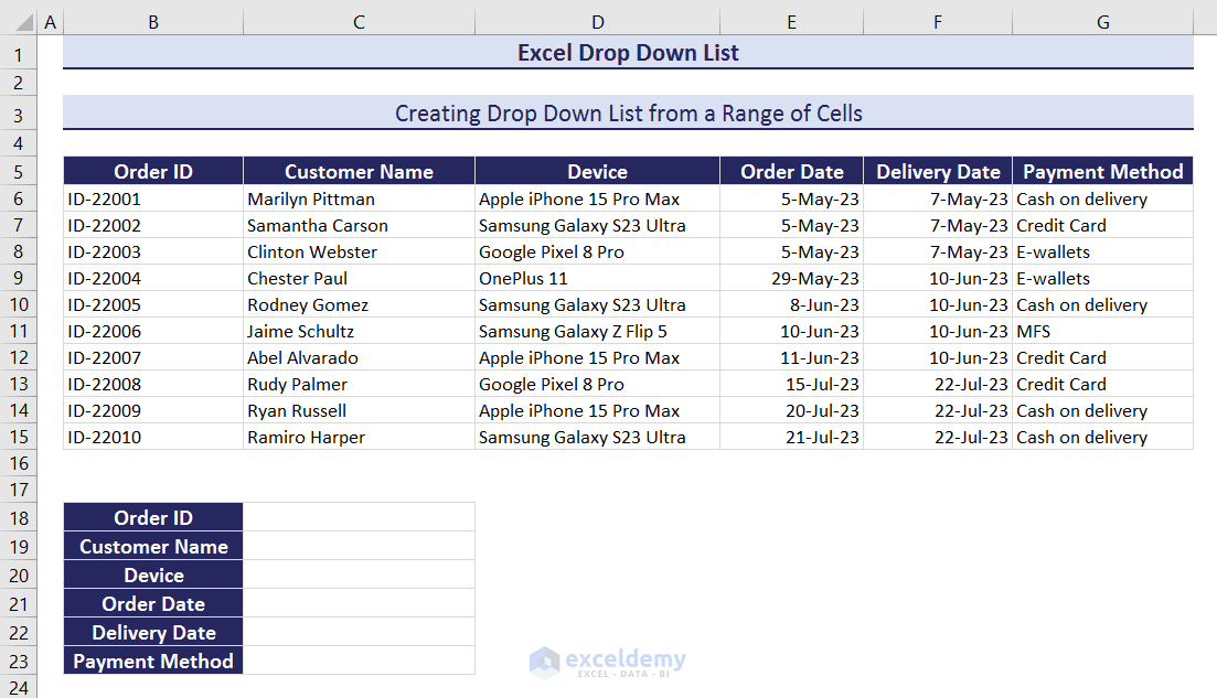
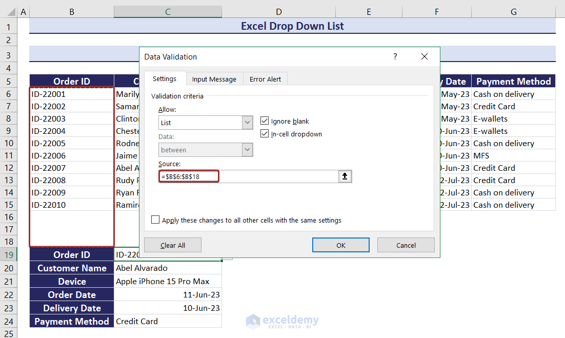
Using a range of cells is one of the most common ways of creating a drop-down list. In the following dataset, I have a dataset regarding a few products’ online purchases. Here, my main target is to create a drop down list based on values in column B under ‘Order ID” header and extract information based on the value selected from the drop down list.
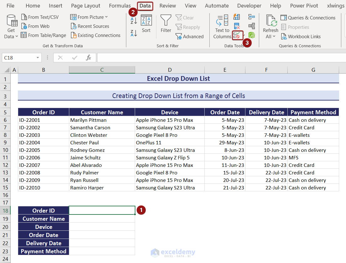
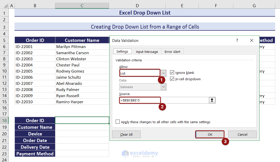
- Select a cell (i.e. C18) to create a drop down.
- Go to the Data tab and select the Data Validation option from the ribbon.
- A wizard named Data Validation will appear.
- From the Setting tab, pick the List option from the Allow section and define a range (i.e. $B$6:$B$15) from the Source section.
- Click on OK to finish the drop down creation.
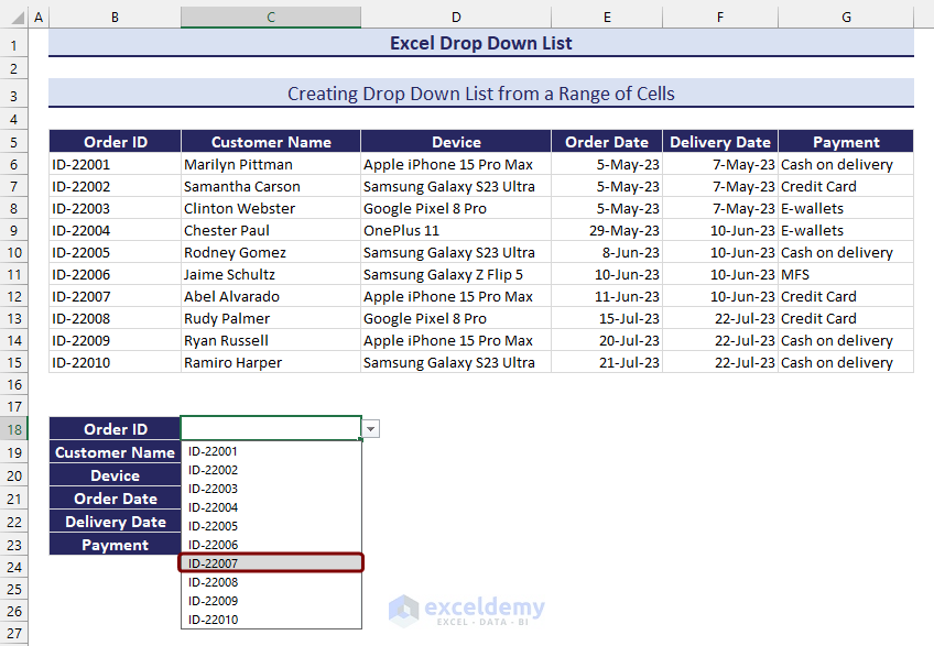
- You will have your drop down list with the values from the range of cells.
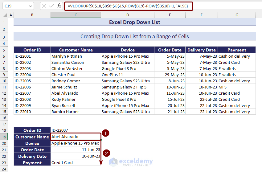
- Now, apply the following formula in cell C19 to have the value from column C under the Customer Name header based on Order ID selection from drop down.
=VLOOKUP($C$18,$B$6:$G$15,ROW(B19)-ROW($B$18)+1,FALSE)- Use Fill Handle to extract values based on the Order ID selection.
2. Creating a Drop Down List from Table
Another simple way of creating a drop down list is by using a table. We can create drop down by defining table column from Data Validation.
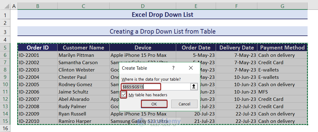
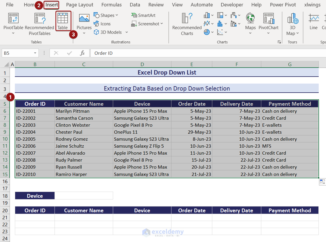
- Select a range of cells and go to the Insert tab to create a table.
- Click on Table from the ribbon.
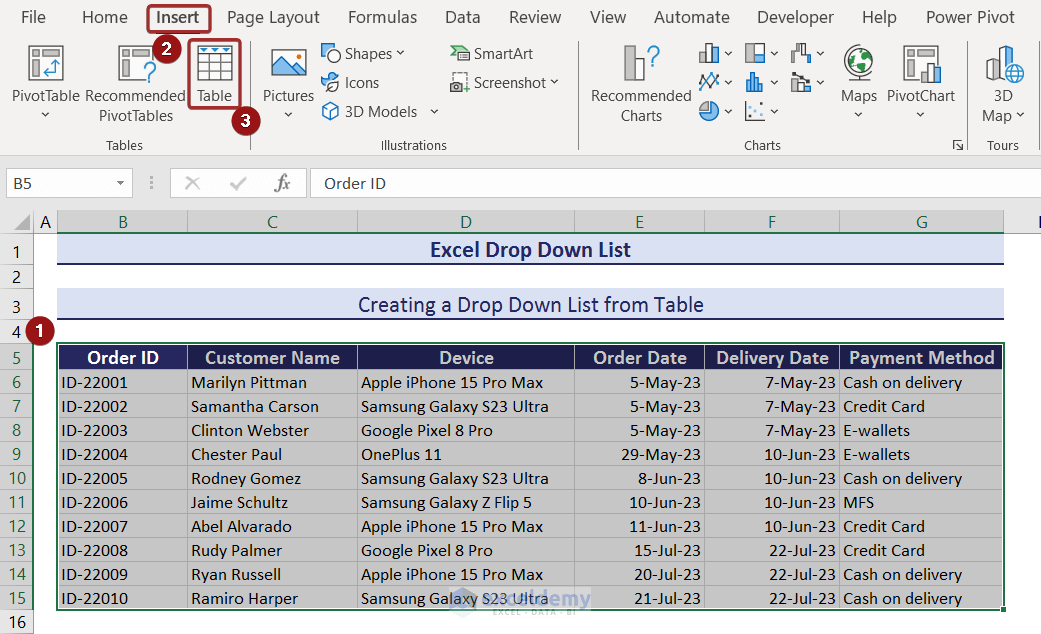
- Confirm the table range and check the box My table has headers.
- Click OK to complete the table completion process.
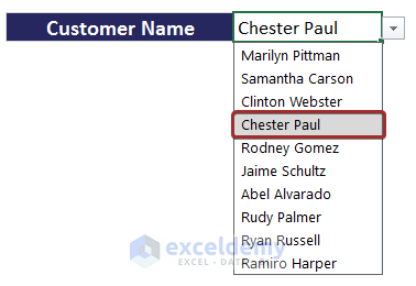
- To create a drop down list in cell C18 with the table column Customer Name, select List from the Allow section.
- Insert the following formula with the INDIRECT function in the Source section and click on OK.
=INDIRECT("Table1[Customer Name]")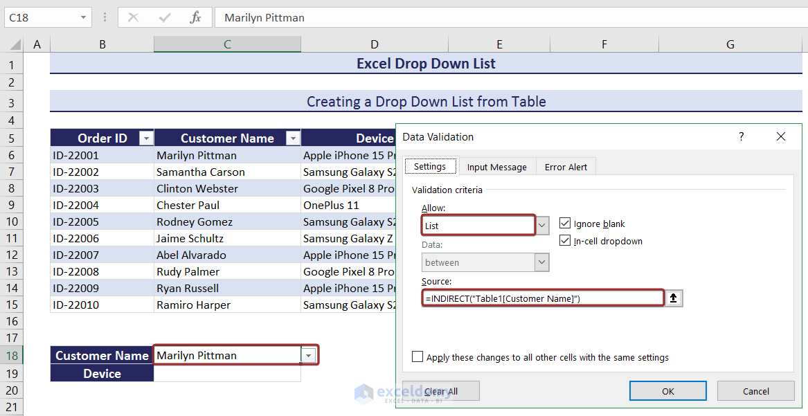
- Now, apply the following formula in cell C19 to extract the device name based on the customer name selection from the drop down.
=INDEX(Table1,MATCH(C18,Table1[Customer Name],0),3)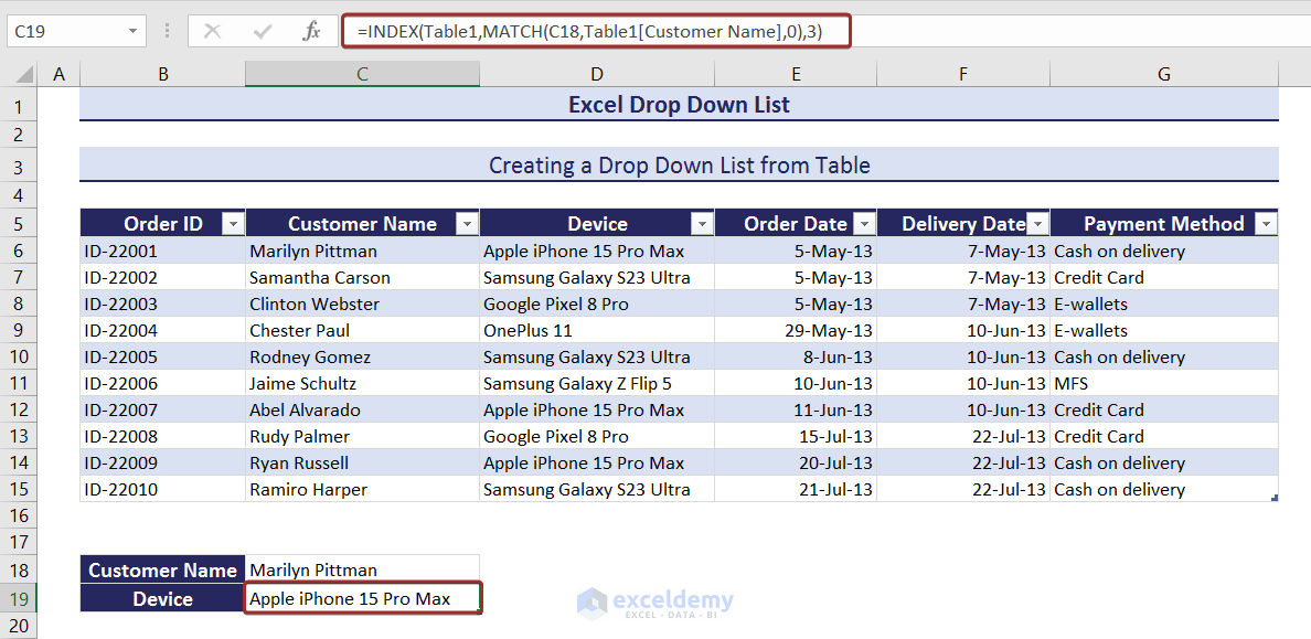
- Thus, we can select a customer name from the drop down and have the device name bought by that customer.
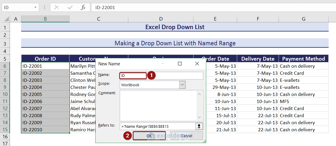
3. Making a Drop Down List with Named Range
We can define a name for a range of cells and use that named range to make a drop down list in Excel.
- Select a range of cells and go to the Formulas tab.
- Click on Define Name from the ribbon.

- Set a name (i.e. ID) from the Name section and define a range from the Refers to section.
- Create a drop down list of order IDs in cell C19 by writing the following formula in the Source
=ID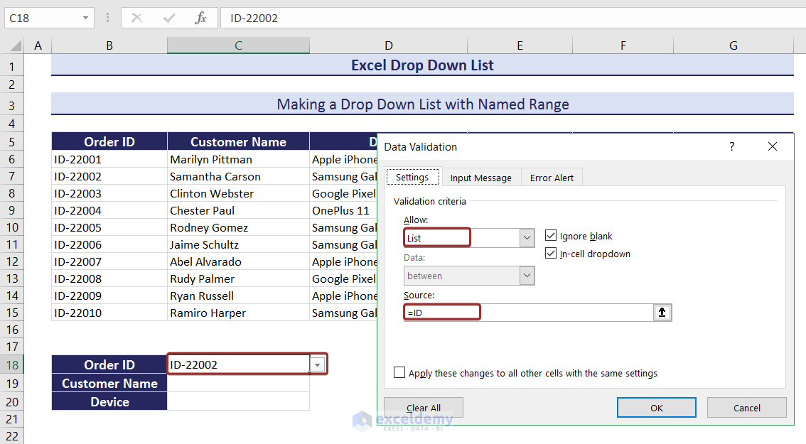
- Apply the following formula in cell C19 to have the customer name based on order ID selected from the drop down.
=INDEX(B6:G15,MATCH($C$18,ID,0),2)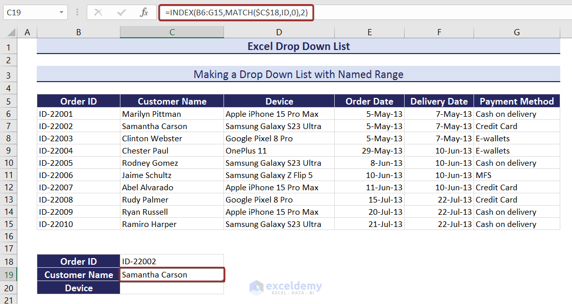
- Again, apply the following formula to have the device’s name in cell C20.
=INDEX(B6:G15,MATCH($C$18,ID,0),3)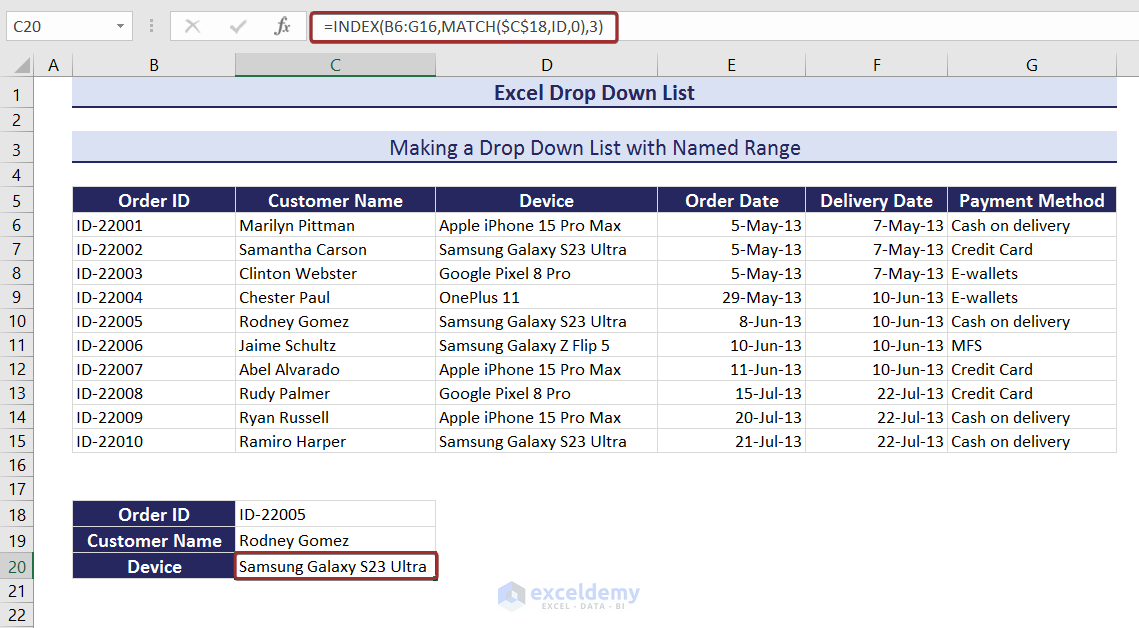
- Thus, we can make a drop down list based on a named range.
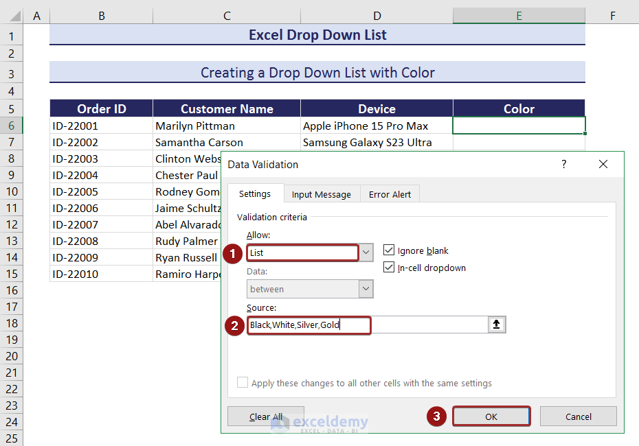
4. Creating a Drop Down List with Color
We can create a drop down list with color where we will define a custom color with Conditional Formatting for each value of the drop down list. In column E of the following dataset, I will define the device’s color and set a cell color accordingly.
- To create a drop down list with a set of color names, select List from the Allow section and write the color names with a comma sign (,) in between the color names (i.e. Black,White,Silver,Gold) in the Source section.
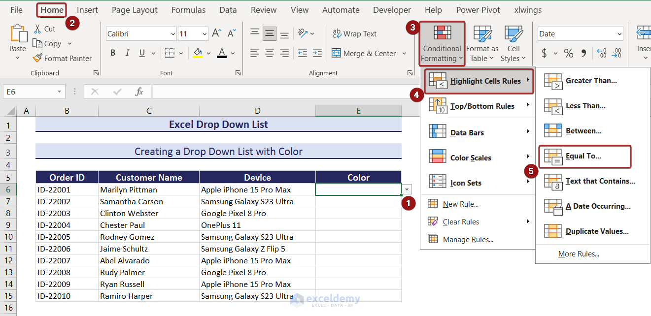
- To define a color for each of the elements of the drop down, select the drop down and go to Conditional Formatting from the Home tab.
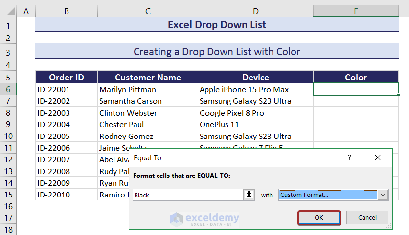
- Go to Highlight Cell Rules and from there, click on Equal To…
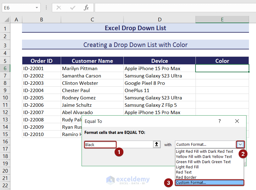
- A wizard named Equal To will appear.
- Write the color name (i.e. Black) and select Custom Format to set a color for that color name.
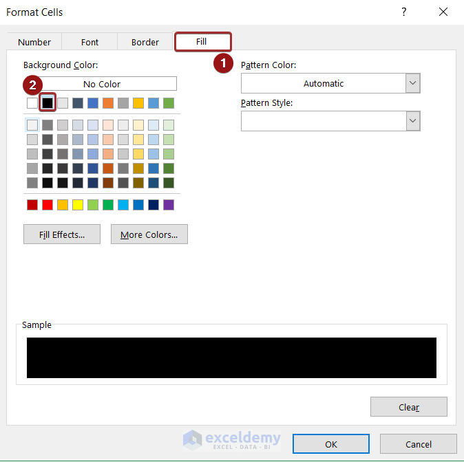
- Pick a color from the Fill tab.
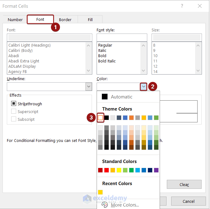
- You can change the font color too from the Font tab. I have set white color for the font.
- Click OK to confirm the formatting.
- In similar ways, set some colors for the other options.
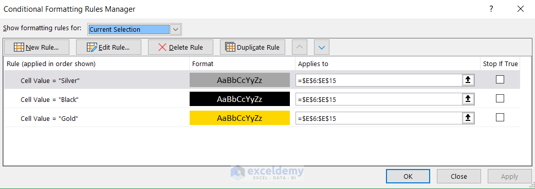
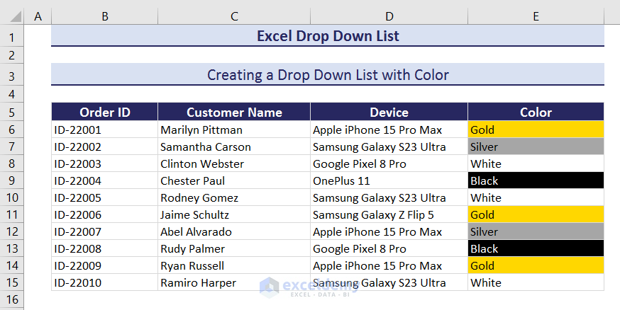
- Now, we will have a drop down with a color based on the cell value.
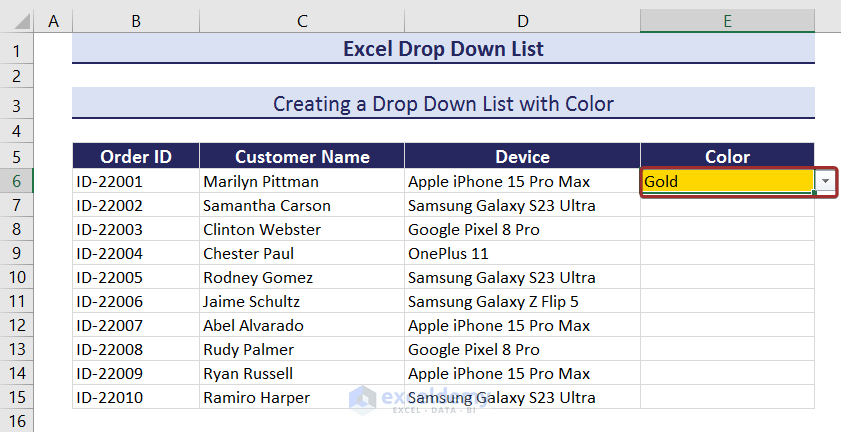
- The cell color will automatically change based on the selection change from the drop down.
- Use Fill Handle to AutoFill this drop down with colors.
5. Making a Drop Down List with Unique Values
With a lot of duplicates in a range of cells, we can create a drop down with unique values ignoring the duplicates. In cell C5, I want to have a drop down with the unique values of column D with the Brand header. I also want to have a drop down with unique values from column E with the Device header that matches the C5 cell value.
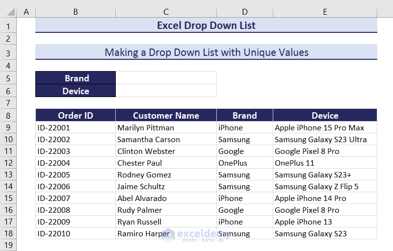
- First of all, apply the following formula with the UNIQUE function in cell B22 to have the unique brand names.
=UNIQUE(D9:D18)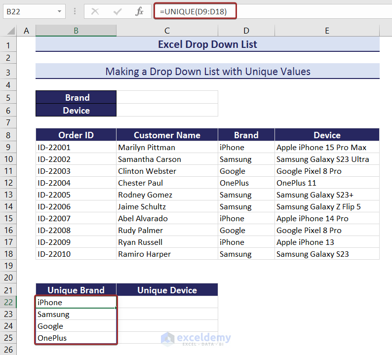
- Now, write the following formula to create a drop down in cell C5 with those unique values.
=$B$22:$B$25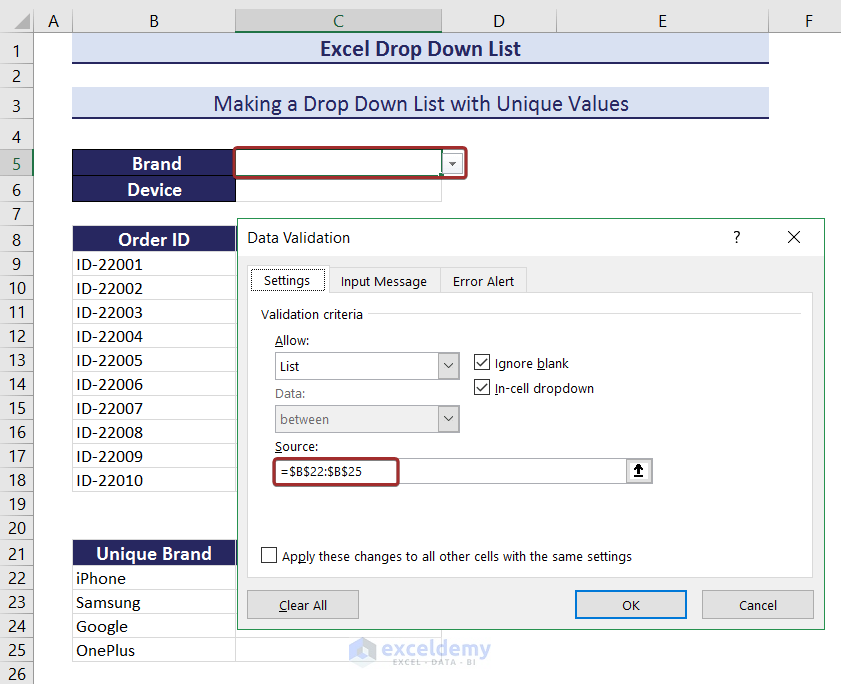
- Now, use the following formula in cell C22 to have the unique values from column E with the Device header that matches the brand in cell C5.
=FILTER(E9:E18,C5=D9:D18)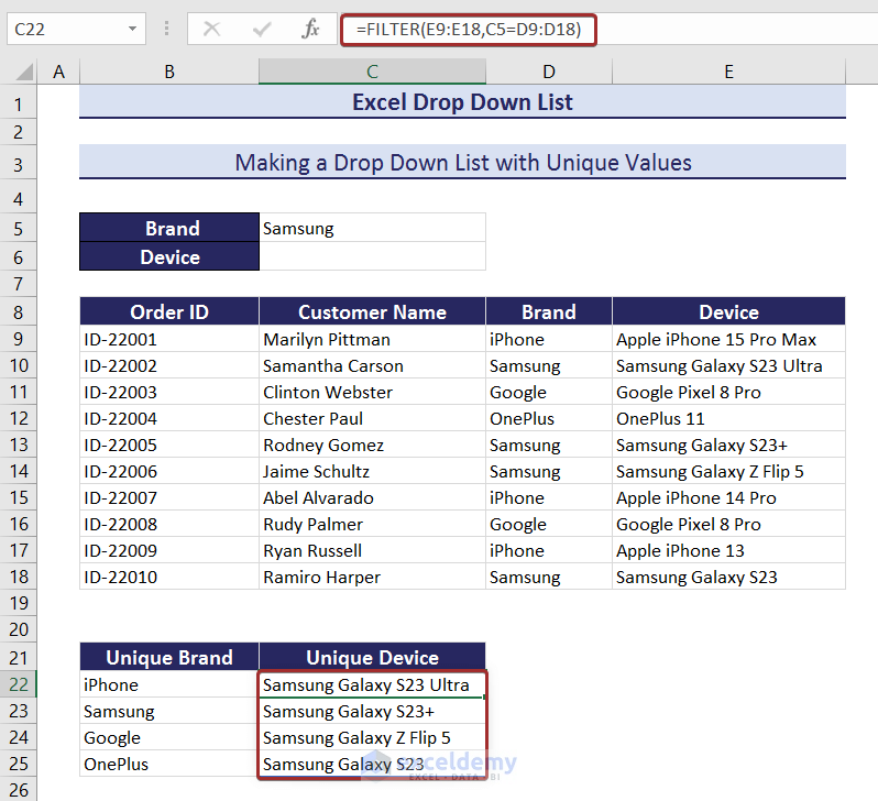
- Now, write the following formula in the Source section of Data Validation to create a drop down with those matched values in cell C6.
=$C$22$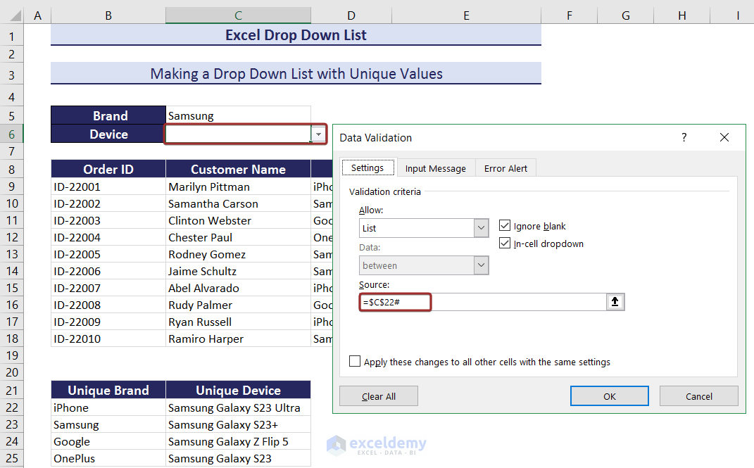
- Thus, we will have a drop down list with unique values.
6. Making a Drop Down List Based on Data from Another Sheet
We can create a drop down list with the data from another worksheet. Here, I have a few mobile brands with their phone models in a worksheet named PhoneList.
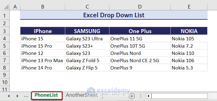
We will use those brand names and phone models to create two drop down list in another worksheet named AnotherSheet.
- To create a drop down list of brand names in cell D6 with the data in the PhoneList worksheet, write the following formula in the Source section of the wizard named Data Validation.
=PhoneList!$B$3:$E$3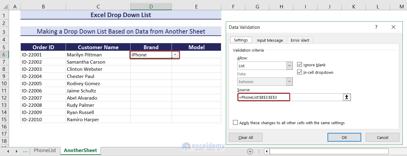
- Use Fill Handle to have the same drop in column D with the Brand header.
- Now, apply the following formula with the INDIRECT function in the Source section to have the phone models from the PhoneList worksheet in a drop down based on the brand names in column D.
=INDIRECT($D6)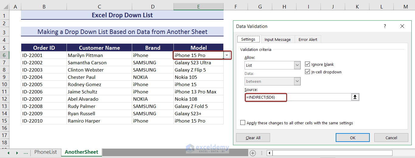
Click here to enlarge the image.
- Thus, we will have a drop down list based on data from another worksheet.
7. Creating a Drop Down List Based on Data from Another Workbook
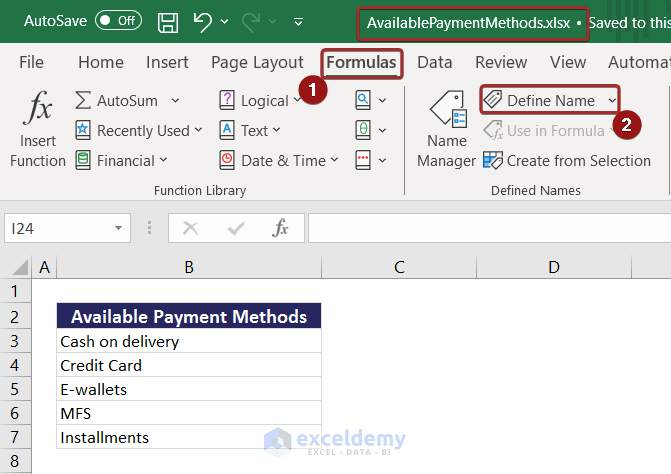
You can make a drop down list based on the data of other workbook. It’s not that complicated though but you have to be careful while doing it. I have a workbook named AvailablePaymentMethods where I have a list of payment methods for online shopping. I will use these data to create a drop down list in the workbook named Drop down in Excel.
- Firstly, go to the Formulas tab and select Define Name from the ribbon to set a name for the range of cells with payment methods.
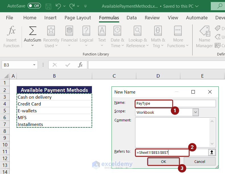
- From the wizard named New Name, define a name (i.e. PayType) from Name and a range (i.e. Sheet1!$B$3:$B$7) from Refers to.
- Click on OK to set the name range.
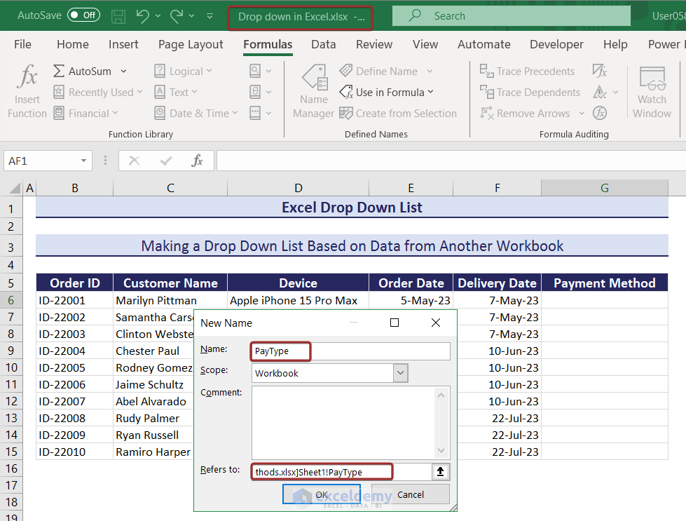
- Now, go to the workbook named Drop down in Excel and set a named range with a name (i.e. PayType) and write [AvailablePaymentMethods.xlsx]Sheet1!PayType to define the previously created name range in the AvailablePaymentMethods workbook.
- Now, write the following formula in the Source section to create a drop down list with that named range in cell G6.
=PayType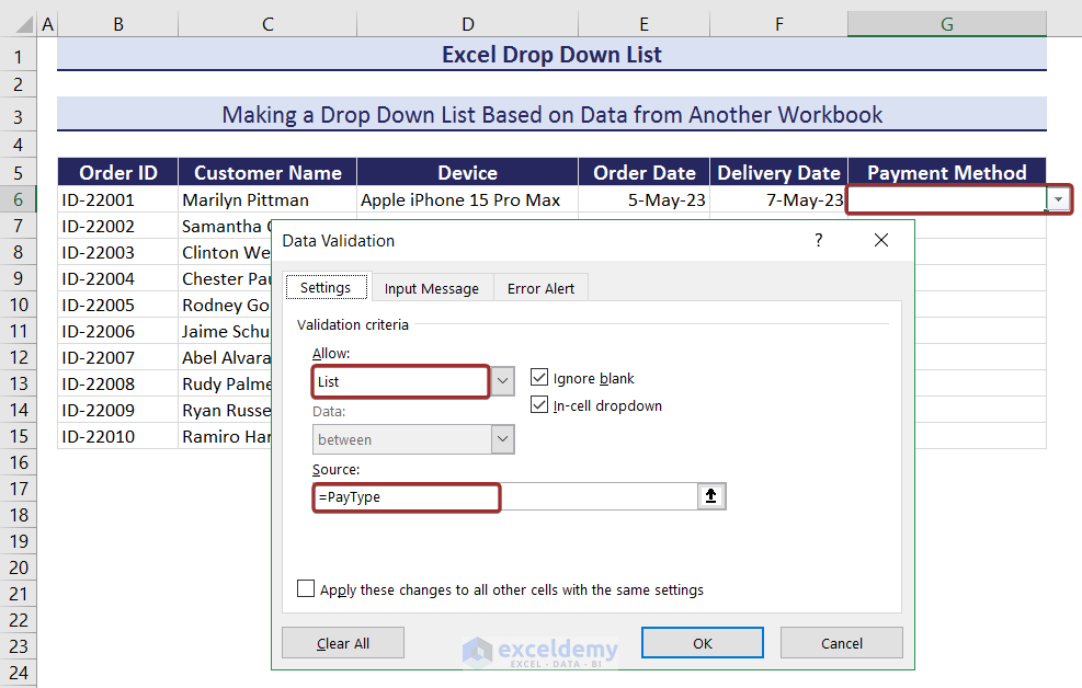
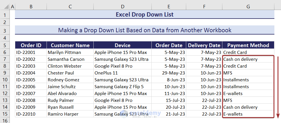
- Finally, we can select a payment method for a customer from the drop down.
- Use Fill Handle to AutoFill the drop down and select a payment method all other customers.
ii. We don’t recommend creating multiple dependent drop down list from another workbook. It’ll need some complex formulas along with complicated procedures.
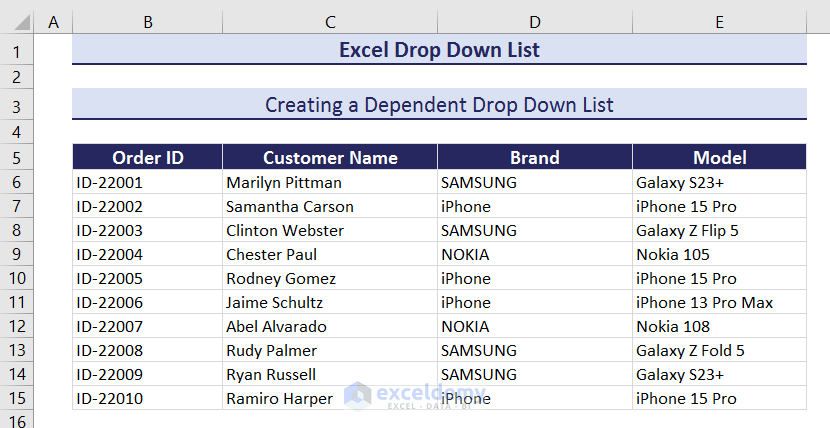
8. Creating a Dependent Drop Down List
We can create a dependent drop list in Excel where the list values will be changed based on the select of another independent drop down list. In the following dataset, I have a list of brands with their phone models. My aim is to create a dependent drop down list of phone models which elements will be changed based on the independent brand value selected from another drop down.
- To create an independent drop down list of brands in cell D6, write the following formula inthe Source section from the wizard named Data Validation.
=$B$18:$E$18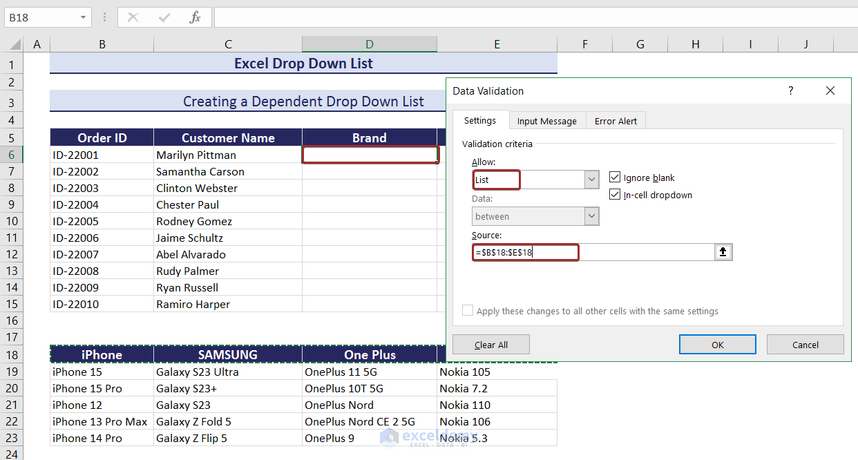
- To create the dependent drop down list of phone models in cell E6, write the following formula with the INDIRECT function in the Source section.
=INDIRECT($D6)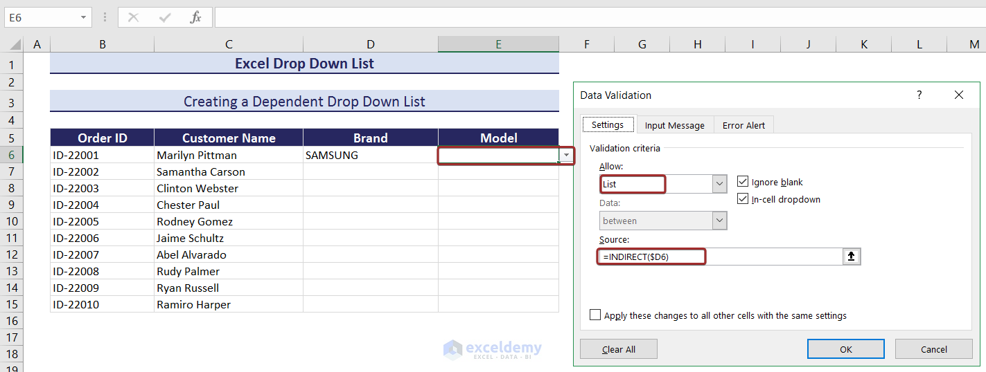
Click here to enlarge the image.
- Now, we will have a dependent drop down based on the selection of brand from an independent drop down.
- AutoFill those drop downs and use it according to your need.
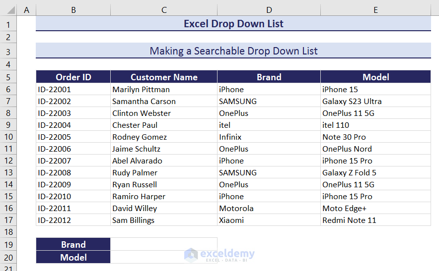
9. Making a Searchable Drop Down List
In a searchable drop down list, we can have an element from a drop down just by searching. From the following dataset, I will create a searchable drop down list in cell C19 with the brand names and there will be a dependable and searchable drop down with phone models in cell C20 based on the selected brand.
- Create new columns in column G and H to have unique brand names and model names and apply the following formula in cell G6 to have unique brand names.
=UNIQUE(OFFSET(D6,0,0,COUNTA(D:D)-1,1))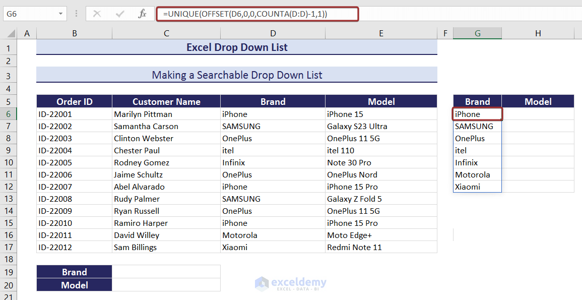
- Now, write the following formula in the Source section to create a searchable drop down in cell C19 with the brand names.
=$G$6#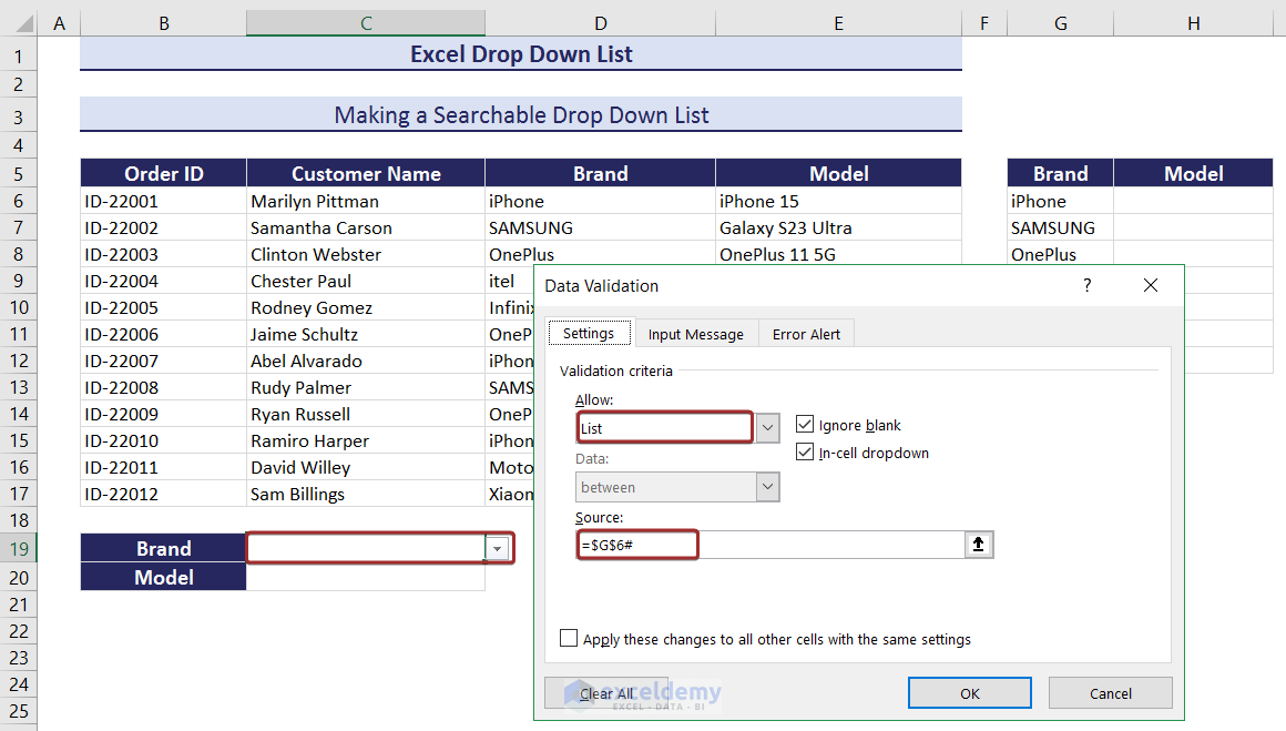
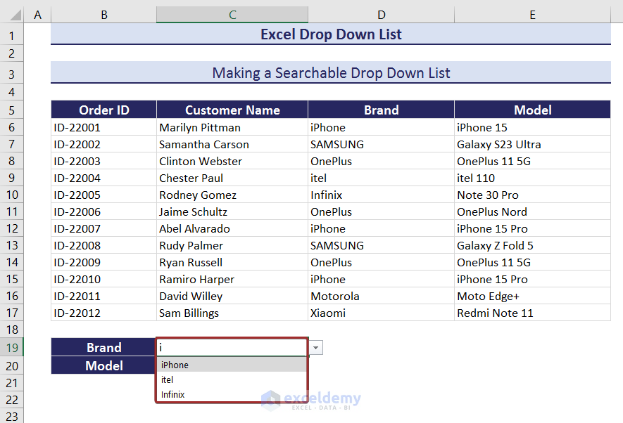
- You will be able to search in cell C19 to have your desired brand name.
- Now, apply the following formula in cell H6 to have phones models based on the brand selected from the searchable drop down.
=UNIQUE(FILTER(E6:E17,C19=D6:D17))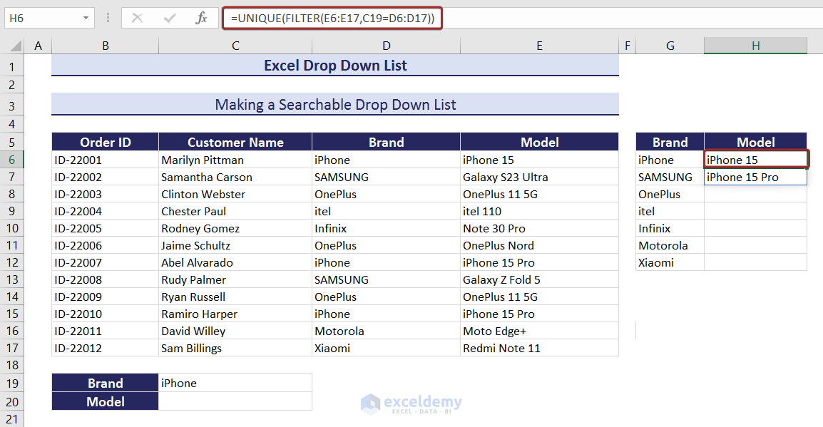
- Similarly, write the following formula in the Source section to create a searchable drop down in cell C20 with the phone model names.
=$H$6#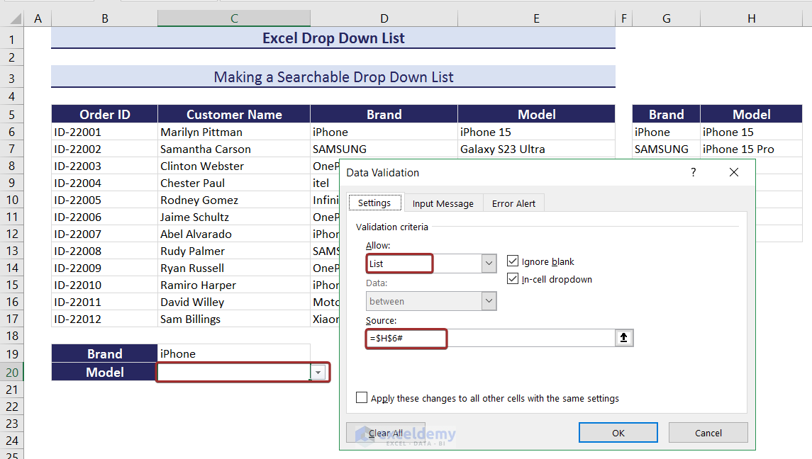
- Now, we have independent and dependent searchable drop down lists.
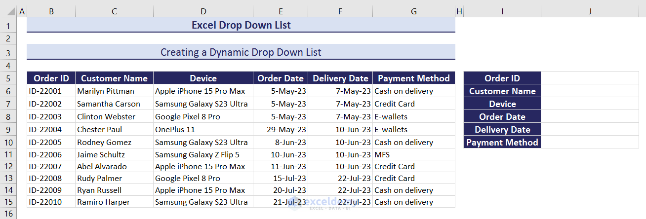
10. Creating a Dynamic Drop Down List to Add & Auto Update New Entries
We can create a dynamic drop down list in Excel where the new entries from a defined column will auto update the drop down list. According to the following dataset, I will create a dynamic drop down based on the values in column B with ‘Order ID’ column header and will extract the values based on that ID.
Click here to enlarge the image.
- Firstly, create a separate column and apply the following formula in cell L6 to have unique IDs regarding column B values.
=UNIQUE(OFFSET(B6,0,0,COUNTA(B:B)-3,1))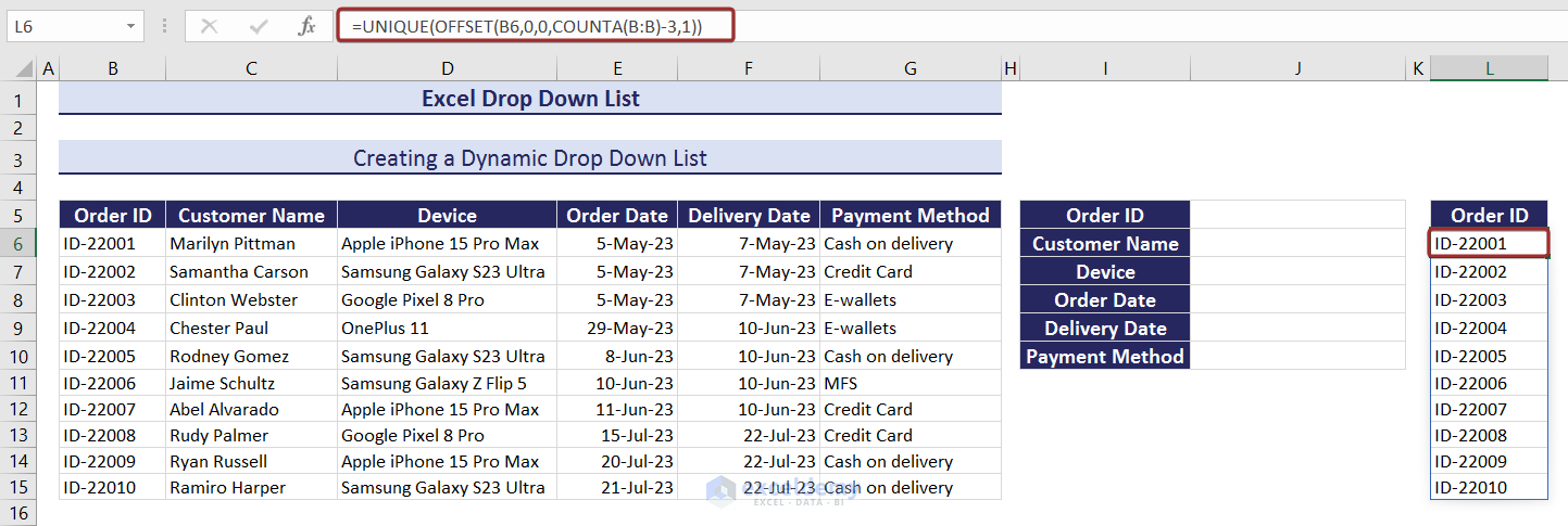
Click here to enlarge the image.
- Now, create a drop down list with those unique IDs in cell J5 by writing the following formula in the Source section.
=$L$6#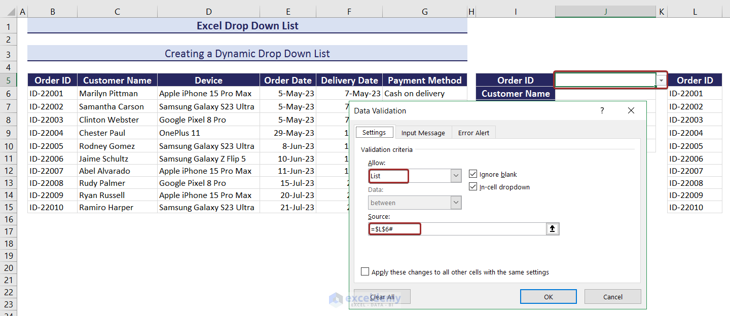
Click here to enlarge the image.
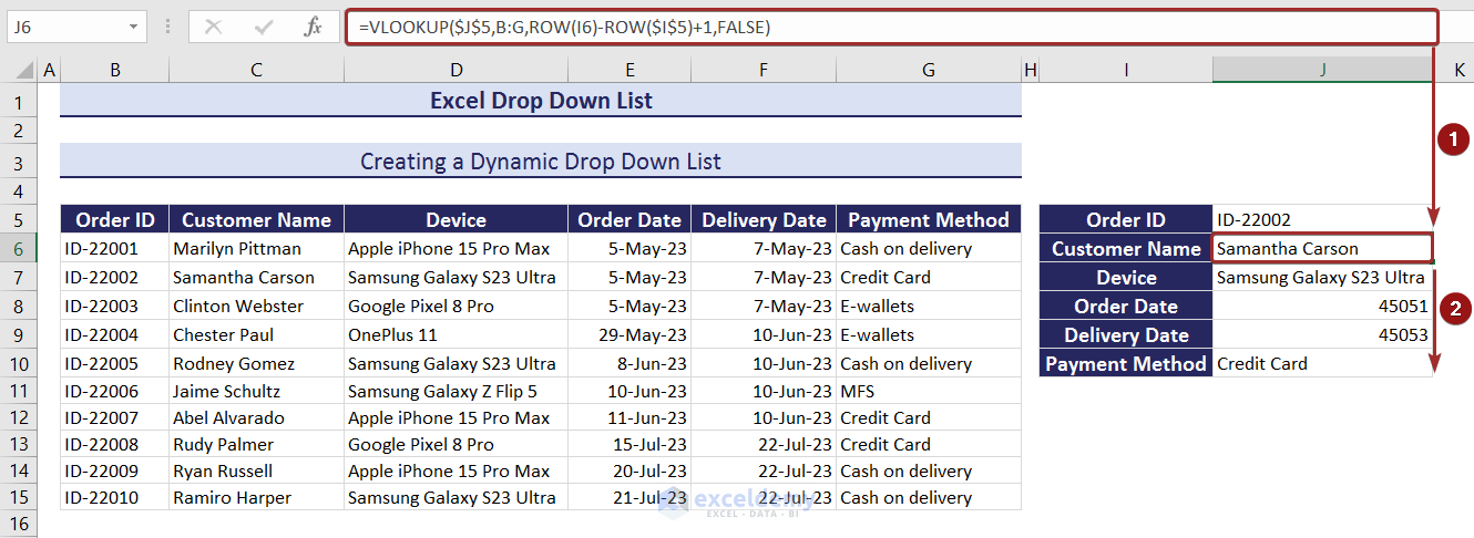
- Now, select an ID from the drop down and apply the following formula in cell J6 to have the customer name of the selected ID.
=VLOOKUP($J$5,B:G,ROW(I6)-ROW($I$5)+1,FALSE)- Use Fill Handle to AutoFill the rest values sequntially regarding that ID.
Click here to enlarge the image.
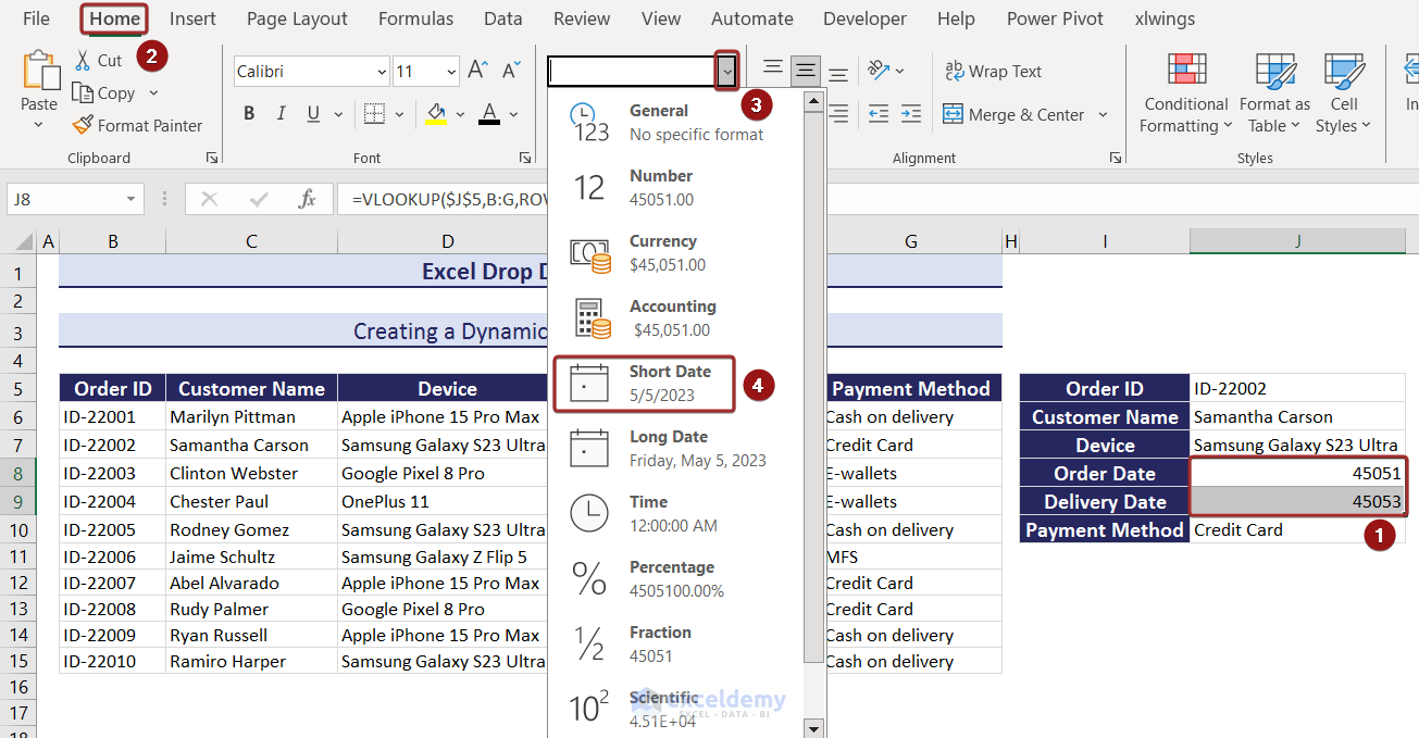
- The extracted dates will be shown as integer numbers. Change the number format to Short Date or Long Date from the Number Format option to regain them as dates.
- Now, if you add extra IDs and their related values in the table, the newly added ID will be automatically updated in the drop down just like in column L.
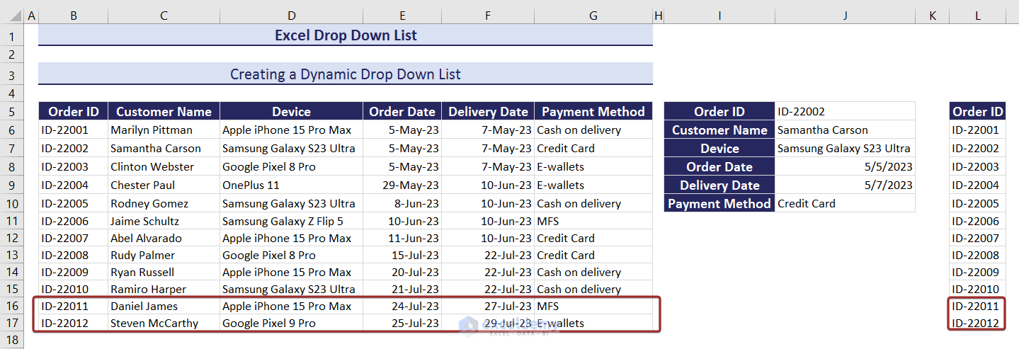
Click here to enlarge the image.
- Pick the newly added values from the drop down and you will have their related data in the defined cells.
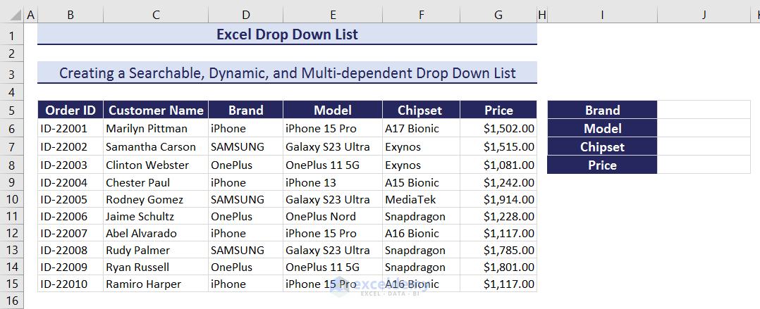
11. Creating a Searchable, Dynamic, and Multi-dependent Drop Down List
It is possible to create a drop down in Excel that will be searchable, dynamic and multi-dependent. Based on the following dataset, I want to create an independent searchable drop down list with brand names, a brand name dependent searchable drop down list of phone models, a phone model dependent searchable drop down list of chipsets and a cell with the price of the product that will be dependent in all of the three drop down lists.
- Apply the following formula in cell L6 to create a dynamic column with unique brand names.
=UNIQUE(OFFSET(D6,0,0,COUNTA(D:D)-1,1))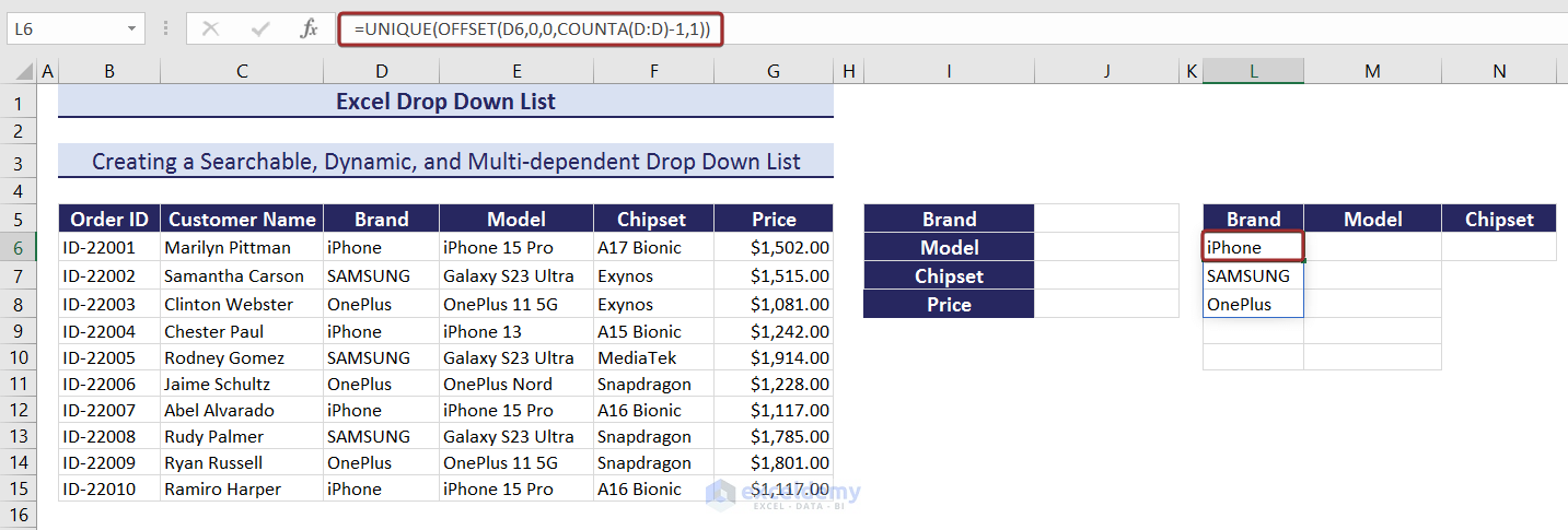
- Now, create an independent searchable drop down of brand names in cell J5 by writing the following formula in the Source section of the wizard named Data Validation.
=$L$6#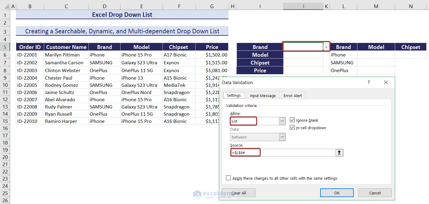
- Next, filter the phone models based on the brand selected from the drop down in cell J5 with the following formula.
=UNIQUE(FILTER(E:E,J5=D:D))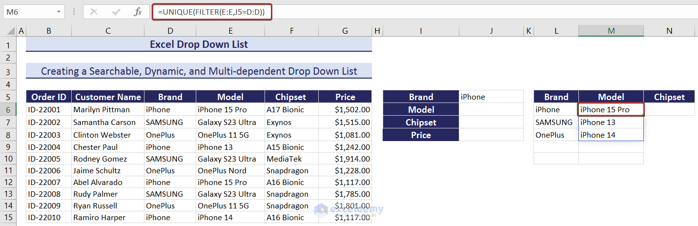
- After that, create an brand name dependent searchable drop down of phone model names in cell J6 by writing the following formula in the Source section of the wizard named Data Validation.
=$M$6#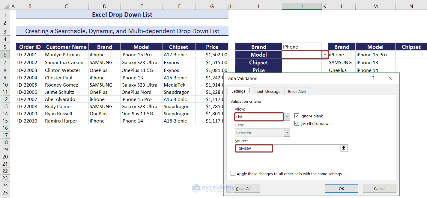
- Similarly, filter the chipsets based on the model selected from the drop down in cell J6 with the following formula.
=UNIQUE(FILTER(F:F,J6=E:E))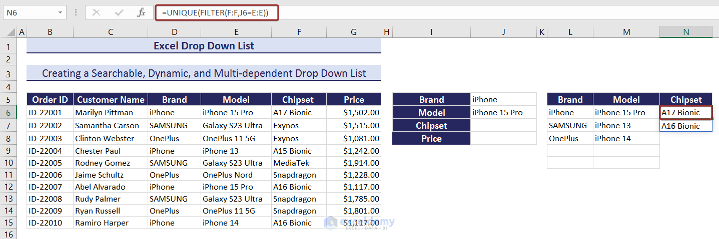
- And write the following formula in the Source section to create a model name dependent searchable drop down of chipsets in cell J7.
=$N$6#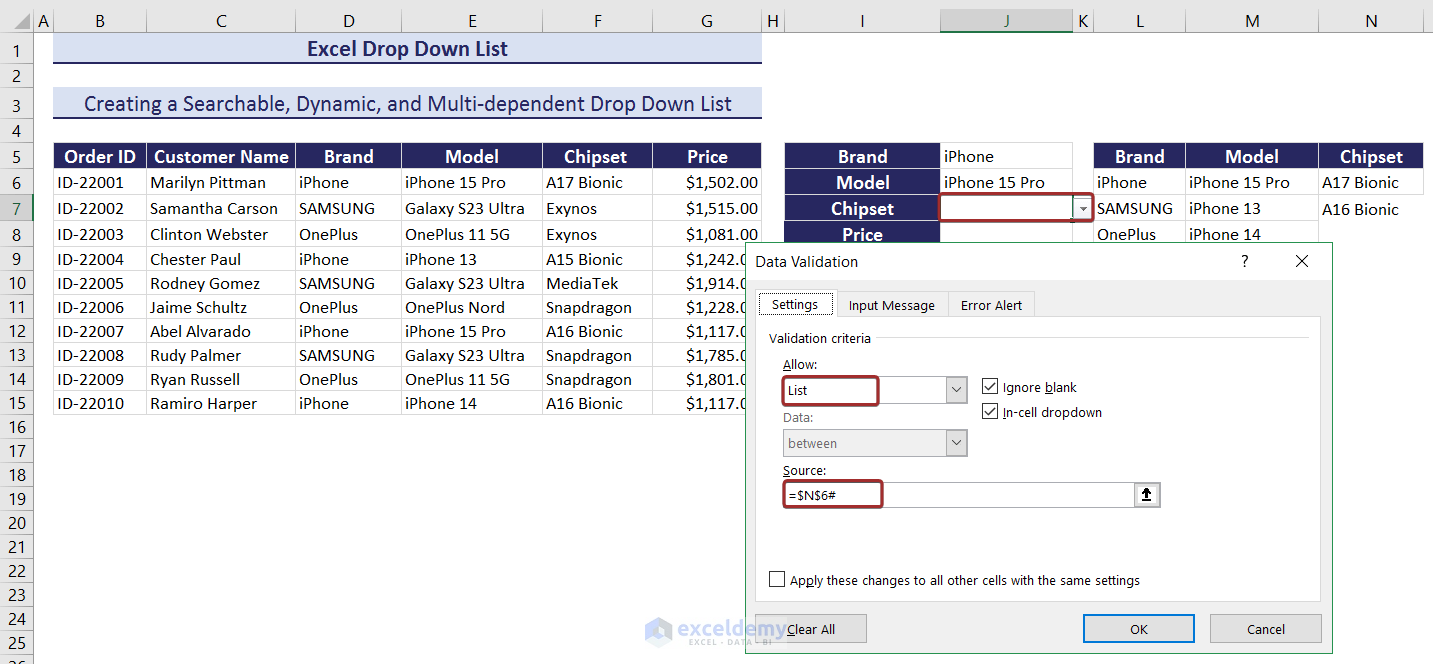
- Now, apply the following formula in cell J8 to find the price of the product that matches all the drop downs’ selected values.
=INDEX(G:G,MATCH(1,(J5=D:D)*(J6=E:E)*(J7=F:F),0))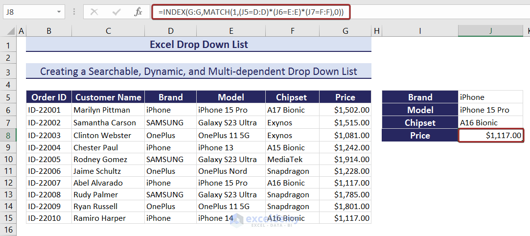
- As all of the drop down lists are dynamic, you can add new entries and find them in the drop down lists.
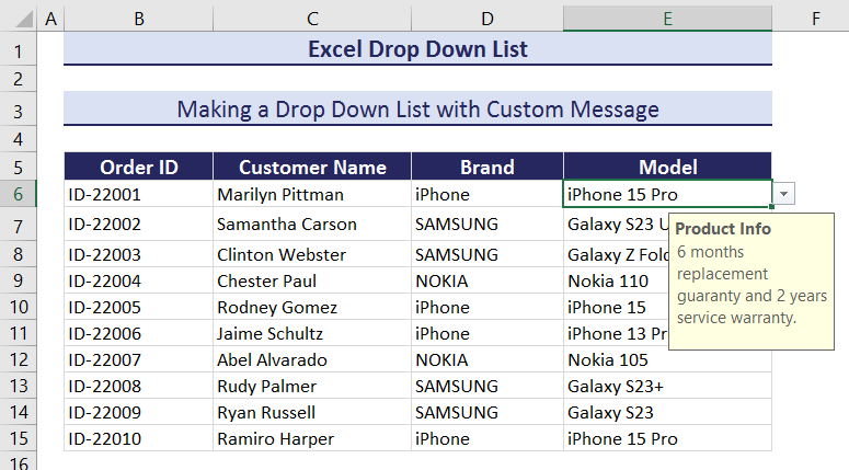
12. Making a Drop Down List with Custom Message
We can fix a custom message with a drop down list. Here, we will try to attach a custom message with the drop downs in column E with the Model header.
- Create a dependent drop down list of phone model like Method-7.
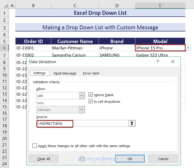
- From the wizard named Data Validation, go to the Input Message tab and check the box named Show input message when cell is selected.
- Set a title from the Title section and a custom message from the Input message section.
- Click on OK to set the custom message with the drop down.
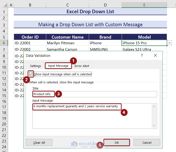
- The custom message will be visible as soon as we select the cell with that drop down.
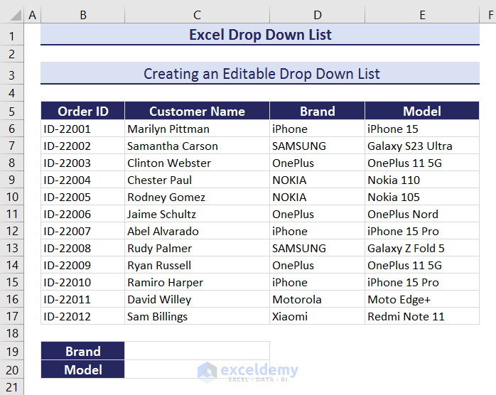
13. Creating an Editable Drop Down List with Error Alert Message
We can also create an editable drop down list in Excel. In a searchable drop down list, we can search for an element that is not listed in that drop down. An editable drop down list will give you multiple chances to edit the search value regarding the drop down list. Here, I have a dataset with online shopping information. I want to create a searchable drop down list of brands in cell C19 and a searchable phone model names based on the selected brand in cell C20.
- Apply the following formula in cell G6 to create a dynamic column with unique brand names.
=UNIQUE(OFFSET(D6,0,0,COUNTA(D:D)-1,1))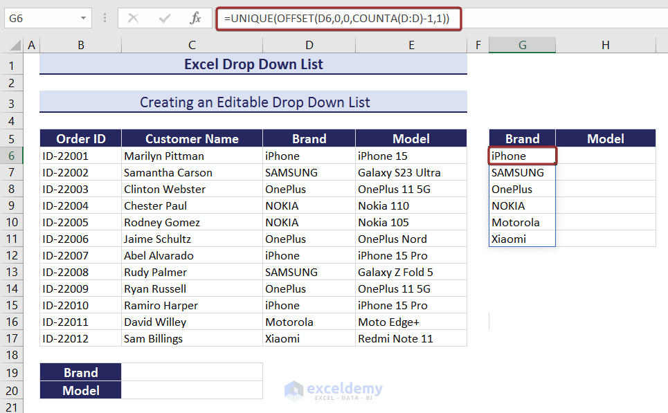
- Now, create a dynamic searchable drop down of brand names in cell C19 by writing the following formula in the Source section of the wizard named Data Validation.
=$G$6#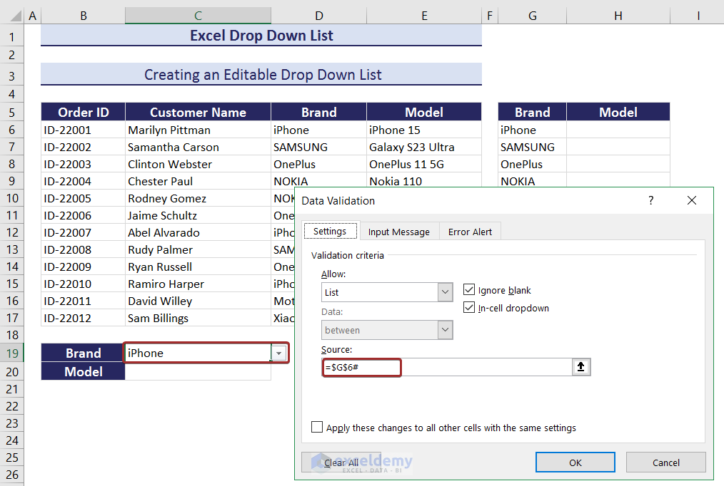
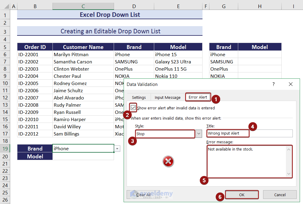
- Now, to make the drop down editable, go to the Error Alert tab and check the box named Show error alert after invalid data is entered.
- Set a style, title, and error message for the wrong search value and click on OK.
- Similarly, creating drop down with the values under Model header.
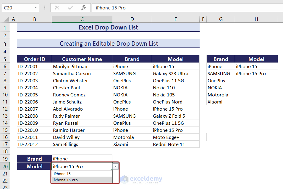
- Now, if you enter any wrong input in those editable drop down lists, it will show the error alert and give you option to retry or cancel.
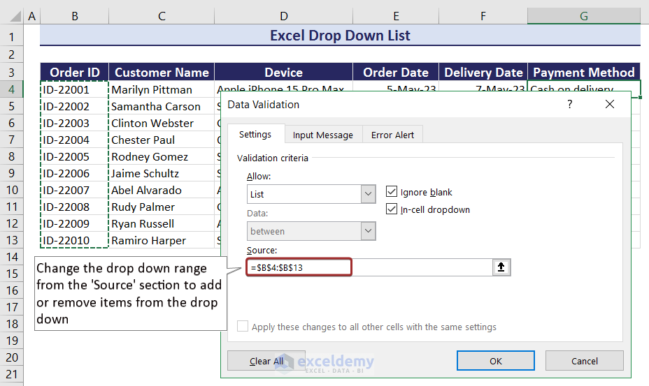
How to Add or Remove Items from Excel Drop Down List?
We can add or remove items from the Excel drop down list just by adding or removing cells while defining range from the Source section.
How to Protect Drop Down List in Excel?
To protect a drop down list in Excel, we need to protect the range of cells used to create that drop down list. In the following dataset, I have created a drop down list of customer names in cell C18. We need to protect the table to protect the drop down.
- Select the entire table and go to the Home tab.
- Click on the button of the Alignment group from the ribbon to extend the Alignment part.
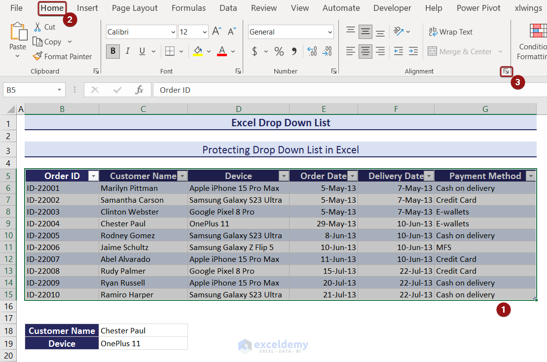
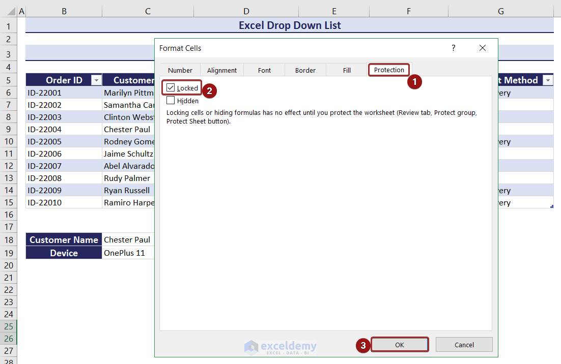
- A wizard named Format Cells will appear.
- Check the Locked option from the Protection tab.
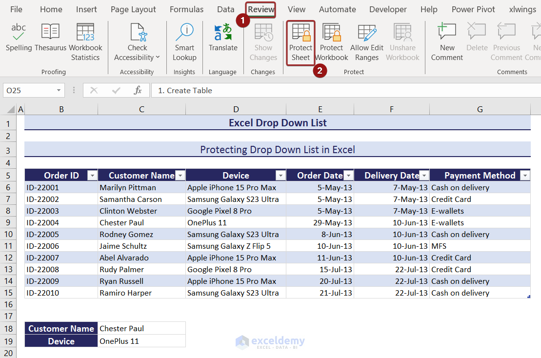
- We have protected the table, but it won’t work till we protect that worksheet or workbook. So, go to the Review tab and click on Protect Workbook from the ribbon.
- Insert a password for protection and check the box named Select locked cells.
- Click OK to move forward.
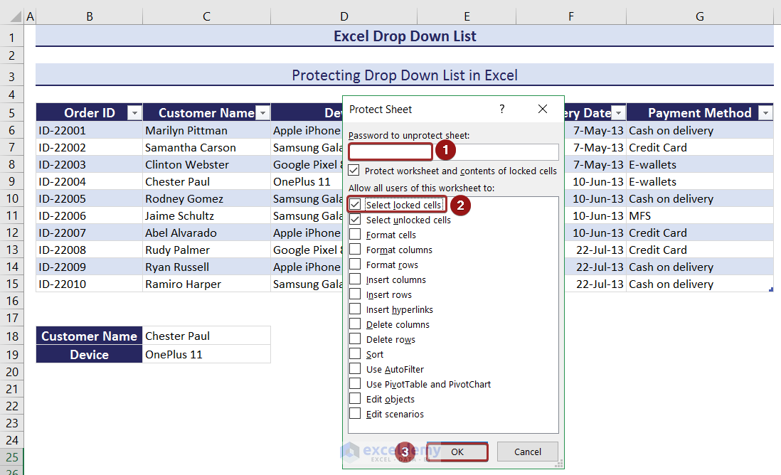
- Re-enter the password for confirmation.
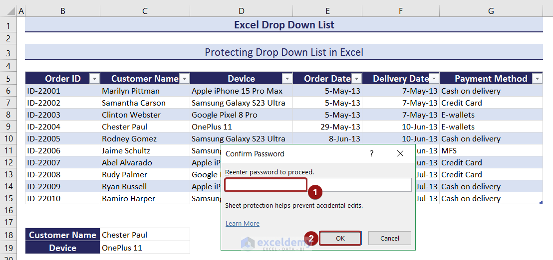
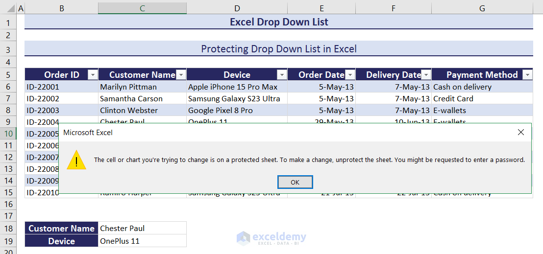
- Now, we have a protected table as well as a protected drop down. So, if you try to change the table range to change the drop down, it will show a warning.
How to Delete Drop Down List in Excel?
We can delete a drop down list in Excel quite easily.
- Select the drop down list and go to the Data tab.
- Click on Data Validation from the ribbon.
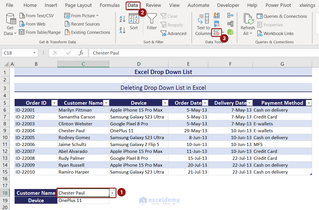
- A wizard named Data Validation will appear.
- Click on Clear All and OK sequentially.
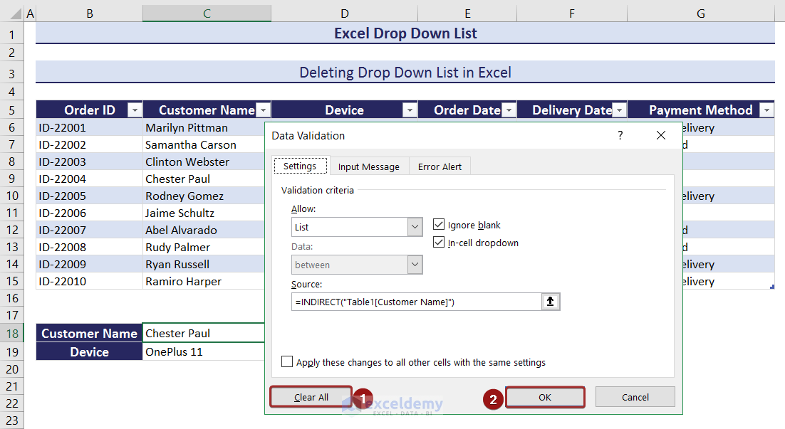
- The drop down list will be removed.
How to Filter Drop Down List & Extract Data Based on Selection in Excel?
We can extract data quite easily based on a drop down selection. For this, create a table first for the given set of data.
Now, create a drop down list from column D named Device of that table.
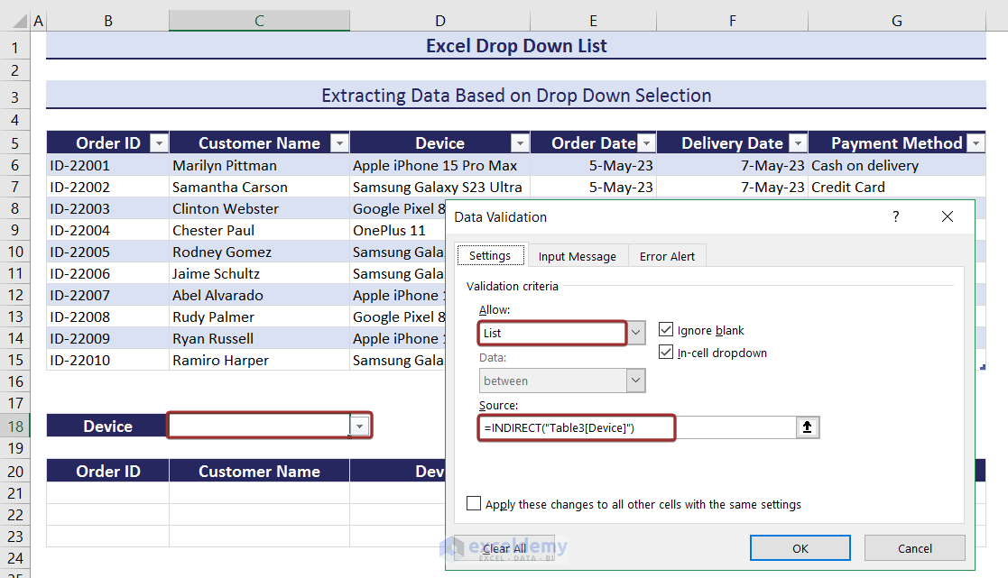
Now, apply the following formula to extract the entire data based on the drop down selection.
=FILTER(Table3,Table3[Device]=$C$18,"No Information Available")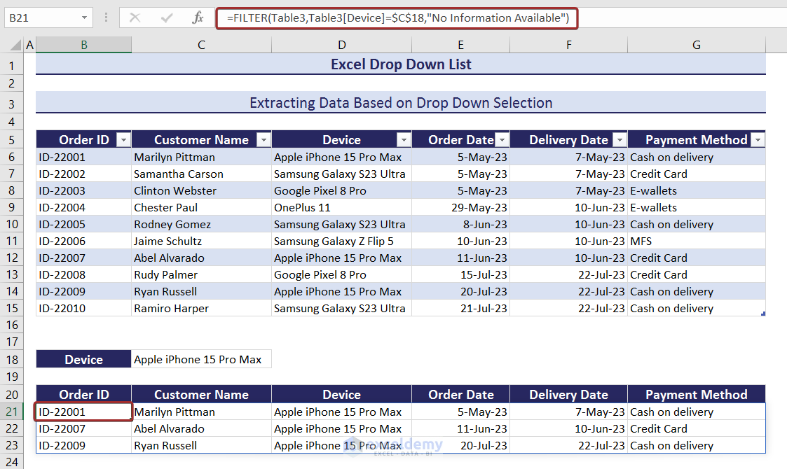
You can change the drop down list’s value and the data extraction will automatically be updated.
How to Solve Issues with Excel Drop Down List?
There might arise a number of issues regarding an Excel drop down list. Every problem has a possible solution.
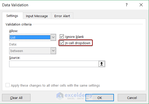
1. Drop Down List Not Visible
The created drop down list might not be visible in a cell if the In-cell dropdown is not checked from the Data Validation wizard.
Solution: Check the box named In-cell dropdown to make the drop down list visible in a cell.
2. Showing Blank in Drop Down List
The drop down list might show blank elements if you do not define the list range properly.
Solution: Define the drop down list range properly to ignore blanks in the drop list.
3. Valid Entries Not Allowed in Drop Down List
If the drop down list is case-sensitive, it won’t allow valid entries that does not match the drop down list cases.
Solution: Use proper cases while entering a valid entry to solve this problem.
4. Invalid Entries Allowed in Drop Down List
Sometimes, the drop down list might allow invalid entries in the drop down. The reason might be defining the wrong range from the Source section in the Data Validation wizard.
As the source range is bigger than the actual value list, the values entered in those cells might get listed even though they are invalid.
Solution: Define the drop down list range properly to stop the entry of the invalid elements in the drop list.
Download Practice Workbook
You can download the practice workbook and try it yourself.
In this article, you have learned the processes of creating a drop down list from a range of cell, from a table, from name range. We have also learned the drop down list creation process from another worksheet and from another workbook. We have also learned the procedures of creating a dependent drop down list, searchable drop down list, dynamic drop down list, editable drop down list, etc. We have also discussed the protection and deletion processes of an Excel drop down list.
Excel Drop Down List: Knowledge Hub
- Create Drop Down List in Excel
- Edit Drop Down List in Excel
- Drop Down List with Filter in Excel
- Excel Dependent Drop Down List
- How to Remove Drop Down List in Excel
- How to Link a Cell Value with a Drop Down List in Excel
- Excel Drop Down List Not Working
- IF Statement to Create Drop-Down List in Excel
- Extract Data Based on a Drop Down List Selection in Excel
- Populate List Based on Cell Value in Excel
- Drop Down List in Multiple Columns in Excel
- Blank Option to Drop Down List in Excel
- Select from Drop Down and Pull Data from Different Sheet
- [Fixed!] Drop Down List Ignore Blank Not Working in Excel
- Autocomplete Data Validation Drop Down List in Excel
<< Go Back to Data Validation in Excel | Learn Excel