In this article, we have discussed different examples of tracker in Excel. You will see the step-by-step process of creating a task tracker. You will get to know about real-time trackers, workflow trackers and progress trackers as well. Finally, we have provided some useful templates of trackers for you.
A tracker can be used for many purposes such as project management, inventory management, event planning, data organizing, employee tracking and so many more. The versatility and flexibility of Excel make it a handy tool to create any type of tracker.
![]()
Download Practice Workbook
You can download this practice workbook while going through the article.
How to Create a Tracker in Excel
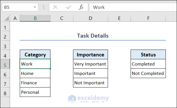
We will show you the step-by-step process to create a tracker in Excel. Here, we have some information about some tasks. We have the category, importance, and status of those tasks. Follow the steps below to create a task tracker in Excel.
- Put the tasks serially in range C5:C14.
![]()
- Select range D5:D14 >> go to the Data tab >> choose Data Validation from the Data Tools group.
![]()
- Set the Data Validation dialog box as shown below. Put this formula into the source bar.
='Task Details'!$B$5:$B$8
- You will see a drop-down box in all the cells of the Category column.
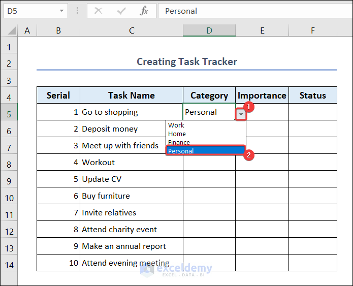
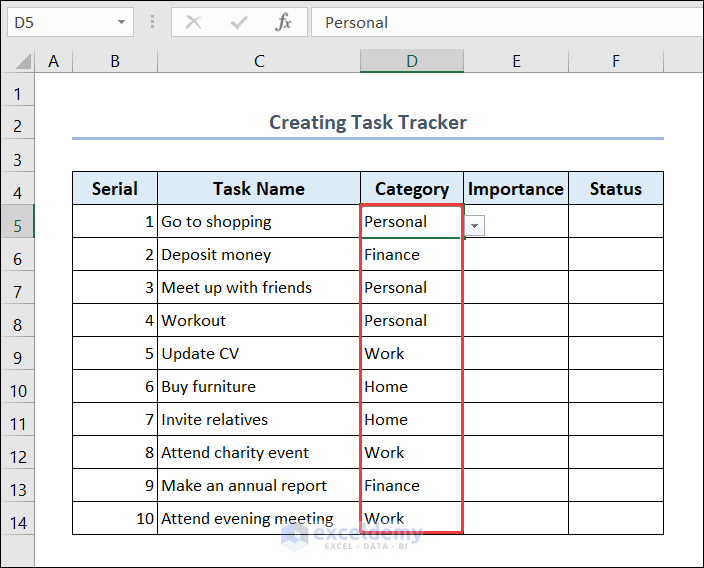
- Use the drop-down box and fill up all the cells of the Category column.
- Repeat these steps and perform Data Validation for the Importance and Status columns. The source bar in the Data Validation dialog box will have different formulas.
Source formula of Data Validation for Importance Column:
='Task Details'!$D$5:$D$7![]()
Source formula of Data Validation for Status Column:
='Task Details'!$F$5:$F$6![]()
- Now fill up range E5:F14 with the help of the drop-down boxes and complete the task tracker.
![]()
- You can get information about a particular task. Put the Serial of the task in cell C4.

- Put these formulas based on the VLOOKUP function in range C5:C8 to see the information of the task.
Formula in cell C5:
=VLOOKUP($C$4,'Task Tracker'!B5:F14,2)Formula in cell C6:
=VLOOKUP($C$4,'Task Tracker'!B5:F14,3)Formula in cell C7:
=VLOOKUP($C$4,'Task Tracker'!B5:F14,4)Formula in cell C8:
=VLOOKUP($C$4,'Task Tracker'!B5:F14,5)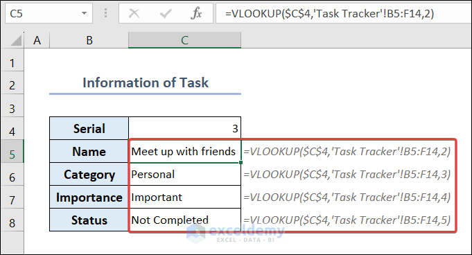
- You can create a task summary as well. Go to cell C5 and put this formula based on the COUNTIFS function.
=COUNTIFS('Task Tracker'!$D$5:$D$14,Summary!$B5,'Task Tracker'!$F$5:$F$14,Summary!$C$4)- Use Fill Handle to AutoFill data in range C6:C8.
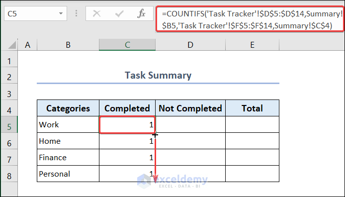
This formula will count the number of cells only. If the value in cell B5 (Work) and cell C4 (Completed) of the Summary worksheet matches any value in range D5:D14 and range F5:F14 in the Task Tracker worksheet respectively.
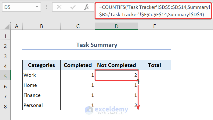
- Go to cell D5 and put this formula based on the COUNTIFS function.
=COUNTIFS('Task Tracker'!$D$5:$D$14,Summary!$B5,'Task Tracker'!$F$5:$F$14,Summary!$D$4)- Select cell D5 and use Fill Handle to AutoFill data in range D6:D8.
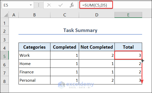
- Go to cell E5 and put this formula based on the SUM function.
=SUM(C5,D5)- Select cell E5 and use Fill Handle to AutoFill data in range E6:E8.
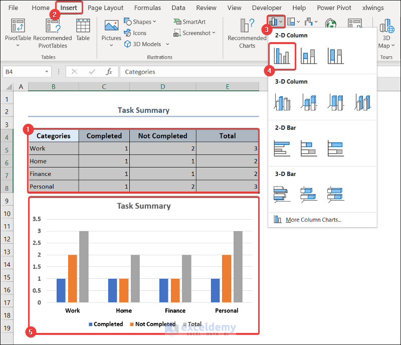
- Now select range B4:E8 >> go to the Insert tab >> select Column Chart option >> choose an appropriate Column Chart.
- You will see a Column Chart with the summary for each category of your tasks.
How to Create Different Trackers in Excel
1. Create a Real Time Tracker in Excel
Design the dataset in the following way.
- Go to cell C4 and put the value of hourly payment in it.
- Fill up the Employee ID and Name columns.
![]()
- Select range D7:E16 >> go to the Home tab >> select Time format from the Number group.
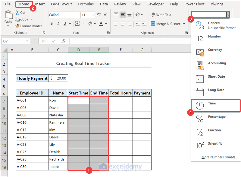
- Fill up the Start Time and End Time columns for each employee.
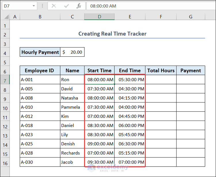
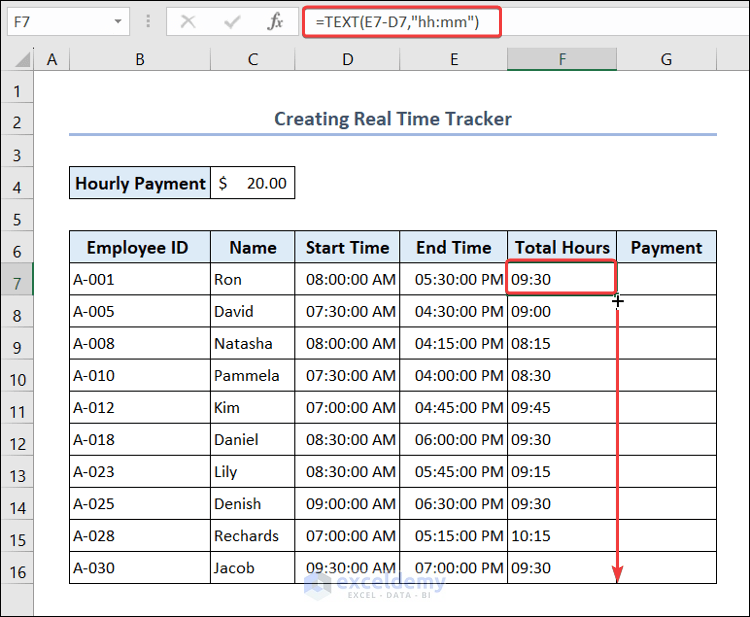
- Go to cell F7 and put this formula based on the TEXT function.
=TEXT(E7-D7,"hh:mm")- Select cell F7 and use Fill Handle to AutoFill data in range F8:F16.
=HOUR(F7)*$C$4+(MINUTE(F7)*$C$4)/60- Select cell G7 and use Fill Handle to AutoFill data in range G8:G16.
![]()
2. Create Workflow Tracker in Excel
We will use the following format to create the workflow tracker.
![]()
- Go to cell E5 and put this formula.
=D5-C5- Select cell E5 and use Fill Handle to AutoFill data in range E6:E14.
![]()
- Put the actual number of days spent for each task in range F5:F14.
![]()
- Select range G5:G14 >> go to the Home tab >> change the number format into Percentage.
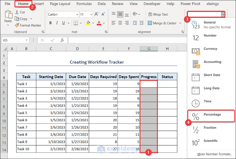
- Go to cell G5 and put this formula.
=F5/E5- Select cell G5 and use Fill Handle to AutoFill data in range G6:G14.
![]()
- Go to cell H5 and put this formula based on the IF function.
=IF(G5=100%,"Complete","In Progress")- Select cell H5 and use Fill Handle to AutoFill data in range H6:H14.
![]()
3. Create a Progress Tracker in Excel
3.1. Use Conditional Formatting
- Follow Method 2 step-by-step to create a progress tracker.
![]()
- Select range G5:G14 >> go to the Home tab >> Conditional Formatting >> New Rule.
![]()
- Set the New Formatting Rule dialog box as shown below.
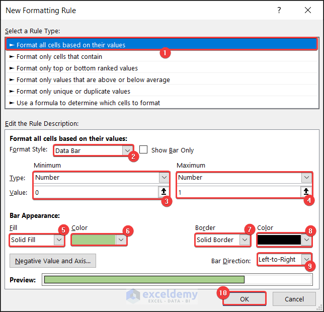
- You will see the progress tracker with data bars in each cell of range G5:G14.
![]()
3.2. Use Bar Chart
We will use the same progress tracker as shown in the previous method.
![]()
- Now select range B4:B14, press the Ctrl button, and select range G4:G14.
- Go to the Insert tab >> select Bar Chart option >> choose an appropriate Clustered Bar Chart.
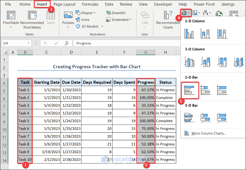
- You will see the bar chart of the progress tracker in your worksheet. You can give it a suitable title.
![]()
3.3. Apply Check Boxes and Circle Chart
We will use the following format to create a progress tracker with check boxes and a circle chart.
![]()
- Select cell D5 >> go to the Developer tab >> click on Insert >> choose Check Box (Form Control).
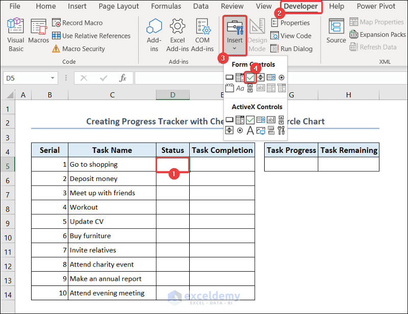
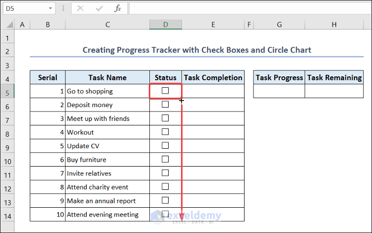
- Create a check box in cell D5.
- Select cell D5 and use Fill Handle to AutoFill to create checkboxes in range D6:D14.
- Right-click on the check box in cell D5 >> select Format Control.
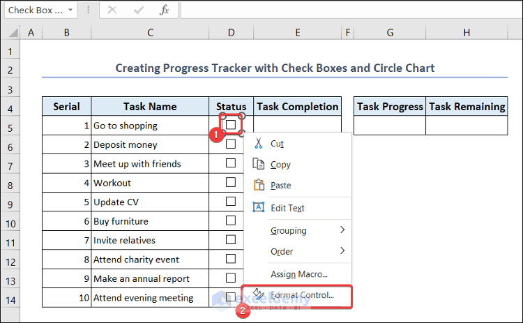
- Set the Format Control dialog box as shown below.
- Insert $E$5 in the Cell Link bar and click OK.
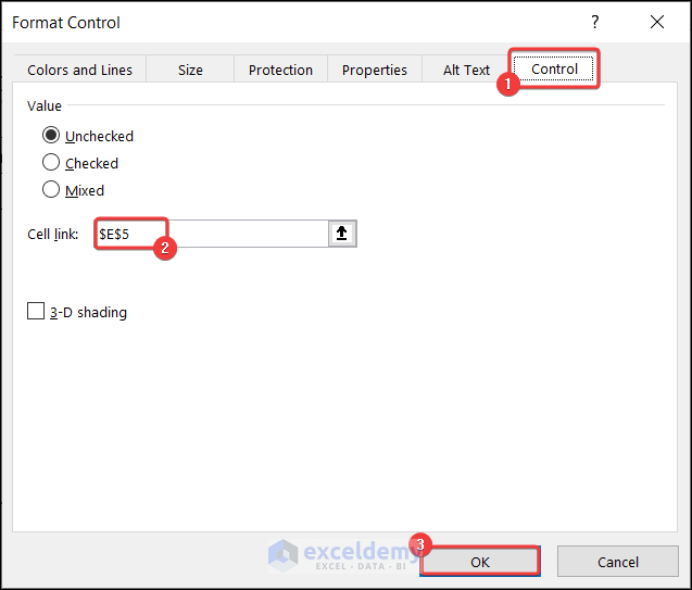
- Now do the same for the rest of the check boxes in range D6:D14 and put the corresponding cell of column E in the Cell Link bar of Format Control dialog box.
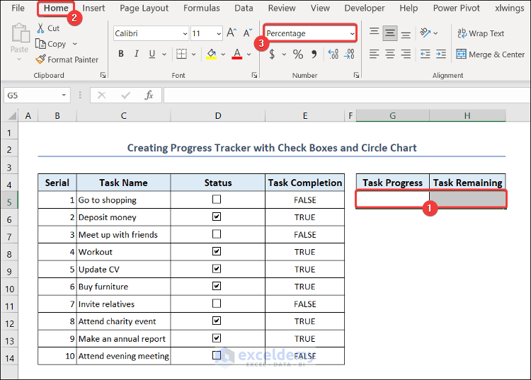
- Tick the check boxes of the completed tasks and you will see TRUE (if checked) or FALSE (if unchecked) in the corresponding cells of the Task Completion column.
![]()
- Now select range G5:H5 and change the number format into Percentage.
=COUNTIF(E5:E14,TRUE)/COUNT(B5:B14)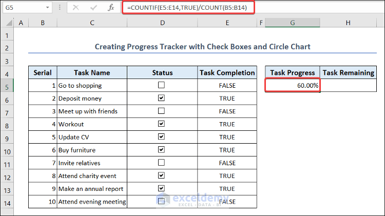
Formula Breakdown
COUNTIF(E5:E14,TRUE): This portion of the formula counts the number of cells in range E5:E14 if any cell value matches the text TRUE.
Result: 6
COUNT(B5:B14): This portion counts the total number of cells in range B5:B14.
Result: 10
COUNTIF(E5:E14,TRUE)/COUNT(B5:B14): This formula returns the percentage of cells that include the text TRUE in range B5:B14.
Result: 60.00%
- Go to cell H5 and put this formula into the cell.
=1-G5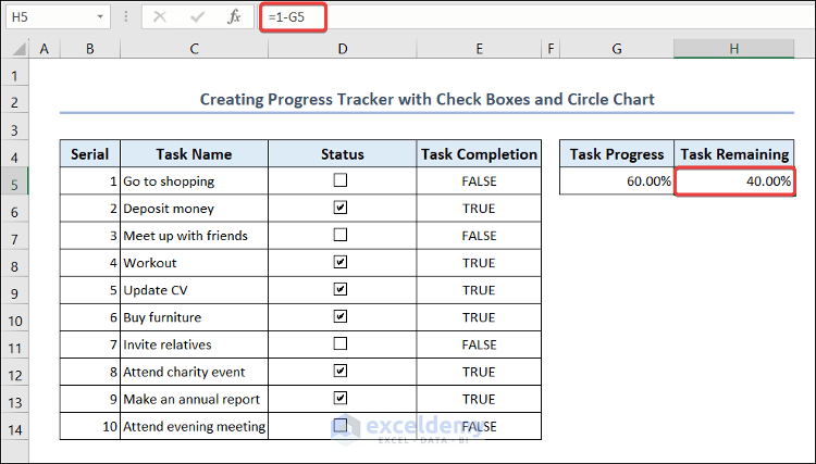
- Select range G4:H5 >> go to the Insert tab >> select the Doughnut chart.
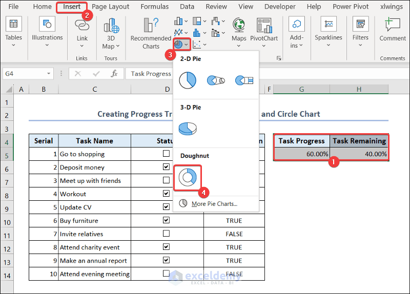
- You will see a circle chart in your worksheet. Give an appropriate title to the chart.
![]()
Templates of Tracker in Excel
1. Inventory Tracker in Excel
You can create an inventory tracker in Excel. An inventory tracker can be used to monitor and manage various company stocks and their whereabouts. It comes with a comprehensive system of recording, tracking, and controlling inventory. This inventory may include different products, materials, or supplies. We have provided an inventory tracker for you.
![]()
2. Project Progress Tracker in Excel
A project progress tracker is a very handy tool in our day-to-day life. You may need a progress tracker for monitoring different activities of your employees in a project and to keep track of their progress. This type of tracker enables companies to have better control and efficiency in managing their employees.
![]()
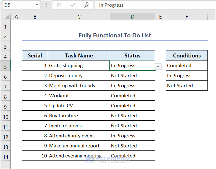
3. Fully Functional To Do List
Excel comes with powerful features and functions to create a fully functional to do list. This list is very flexible and easily customizable. It is very handy and you can use it to keep track of your day-to-day activities.
Things to Remember
- Select the source for Data Validation carefully.
- Select the desired range of cells before setting the Conditional Formatting dialog box.
- Keep your tracker updated.
Frequently Asked Questions
1. What are the best practices for organizing data in an Excel tracker?
You can follow some practices for organizing data in an Excel tracker. You should use consistent headings and group interconnected information together. It is better to use separate sheets or tabs for different sections or categories. You should keep an organized data structure that is easy to understand and navigate.
2. How do I set up data validation to ensure accurate data entry in my tracker?
To set up data validation in Excel follow this:
- Select the cells where you want to apply validation.
- Go to the Data tab.
- Click on Data Validation, and specify the validation criteria such as whole numbers, decimal numbers, dates, or values from a specific list. You can also set custom validation rules to meet your specific requirements.
3. How can I protect my tracker from accidental modifications or unauthorized access?
To protect your tracker,
- Go to the Review tab.
- Click on Protect Sheet or Protect Workbook and set a password to prevent unauthorized modifications.
You can also restrict editing permissions and specify who can make changes to the workbook.
Conclusion
In this article, we have presented different methods to create a tracker in Excel. This article aims to enhance users’ efficiency and productivity when it comes to tracking business inventory, employee activities, etc. If you have any questions regarding this essay, don’t hesitate to let us know in the comments. Also, if you want to see more Excel content like this, please visit our website, and unlock a great resource for Excel-related content.
Tracker in Excel: Knowledge Hub
<< Go Back to Excel Templates

