Excel Optimization with Constraints (3 Case Scenarios)

Get FREE Advanced Excel Exercises with Solutions!

Optimization analysis is a more complex part of goal-seeking analysis for one or more variables based on certain constraints. Even you can change the constraints and control the optimization process. It may sound very complex. But Microsoft Excel has introduced Solver for making such optimization analysis easier. In this article, we will first get to Excel Solver a little more. Then we will describe the process of excel optimization with constraints through 3 case scenarios.

Table of Contents Expand

What Is Excel Solver?

Excel Solver is a kind of What-if analysis tool that holds a special set of commands. It is used for optimization as well as a simulation in many business and engineering models.

Excel Solver is the best tool for optimization with constraints. It helps to determine the return on investments, optimal budget, production cost, scheduling workforce, and lots more.

Types of Methods for Optimization in Excel Solver

There are three methods in solver for optimization. They are as follows:

Simplex LP: In this method, each constraint refers to a linear model requirement. Therefore the target cell is optimized in (changing cell*constant) form and compared to the sums of a constant.
Generalized Reduced Gradient (GRG) Nonlinear: When target cell or constraints or both refer to changing cells, it refers to a nonlinear method for optimization.
Evolutionary: It is quite similar to GRG nonlinear only with the difference that it is used for smooth nonlinear problems.

How to Do Optimization with Constraints in Excel: 3 Case Scenarios

Now, let us learn the process of optimization with constraints in excel solver with the following 3 case scenarios.

1. Optimization with Constraints in Maximize Open Channel Flow

In this case, we will describe constrained optimization by maximizing open channel flow in a trapezoidal cross-section. For this, we will consider 3 variables– Top Width, Height and Angle of side walls. With the help of constraints, we can optimize the flow rate by maximizing the Hydraulic Radius based on the variables. Here, Hydraulic Radius is defined when any cross-sectional area is divided by the Wetted Perimeter (R=A/p). Now, go through the following steps carefully.

In the beginning, provide the Inputs, Values and their Units in the Cell range B5:D8.

Then insert this formula in Cell G5 to calculate the Bottom Width of the trapezoid channel.

=C5-2*C6*(TAN(RADIANS(90-C7)))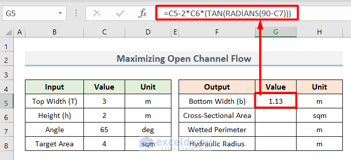

In this formula, we used the RADIANS function to convert the degree angle in Cell C7 to radian and determine the tangent value with the TAN function.

After this, type this formula in Cell G6 to find out the Cross-Sectional area (A).

=C6*(G5+C5)/2

Following this, calculate the value of the Wetted Perimeter (p) with this formula in Cell G7.

=G5+2*SQRT(((C5-G5)/2)^2+C6^2)

Here, we used the SQRT function to get the square root value.

Lastly, get the Hydraulic Radius with this formula in Cell G8.

=G6/G7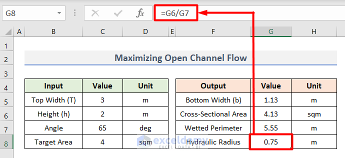

Along with this, determine the units in the Cell range H5:H8 as shown below.

Next, we will add constraints and variables in Excel Solver.
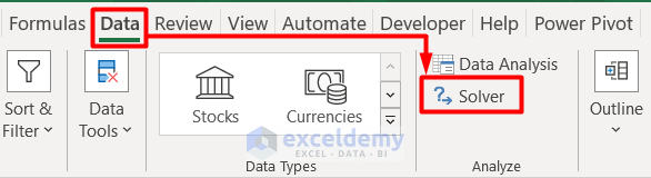
For this, go to the Data tab and choose Solver from the Analyze section.

Here, insert Set Objective as Cell G8 because we will maximize the Hydraulic Radius for optimization.

Then, refer to Cell range C5:C7 as the By Changing Variable Cells because these values will change through optimization.

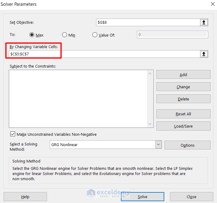
Now, click on Add in the Solver Parameters window.

Following this, insert the Cell Reference and Constraint value as shown below. The constraint value will set up a limit for optimization.

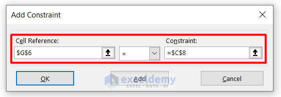
Note: Constraint value can either be a numeric value or a cell reference. But it is a best practice to refer to a cell.

Then, press OK and you will see the conditions in the Subject to the Constraints box.

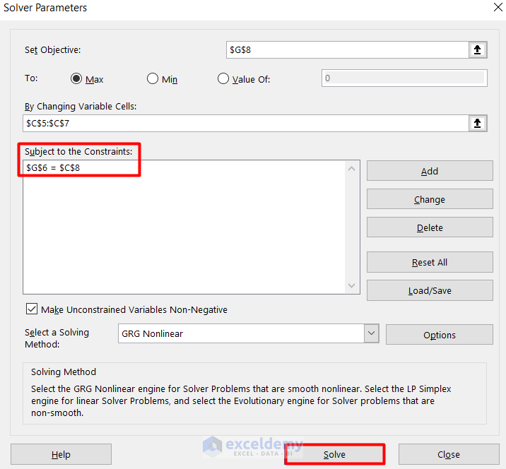
Now, click on Solve and it will direct you to the Solver Results window.
In this window, mark checked the Keep Solver Solution and click OK.

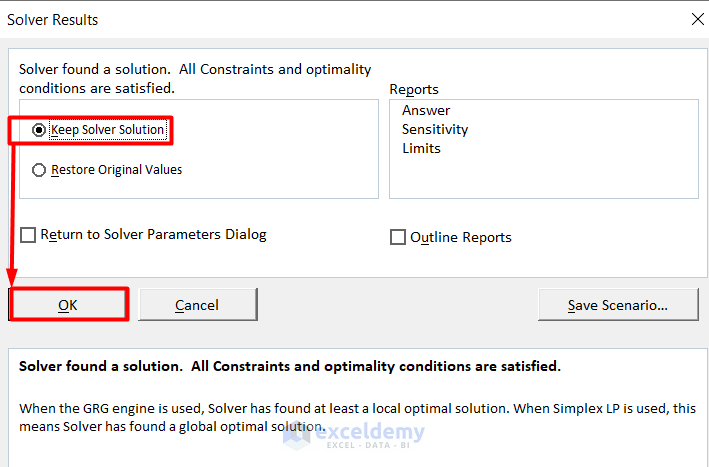
Finally, the values will be optimized because the Target Area and the Cross-Sectional Area are now equal.

It also optimized the Input values of the variable cells based on the constraint.

2. Optimization with Constraints in Linear Programming Problem

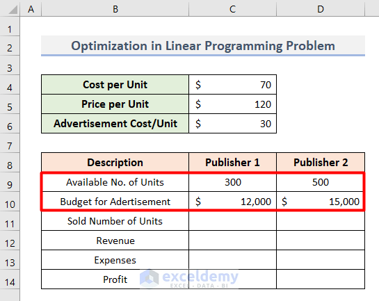
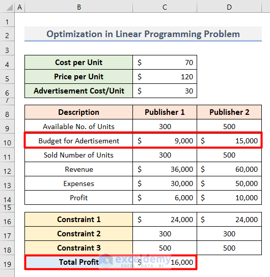
In this second case, we will analyze and optimize the Total Profit of a manufacturing company for advertisement. For this, we will consider 2 Publishers’ Budget for Advertisement as the variables. Follow the process below to optimize this case with constraints as a linear programming problem.

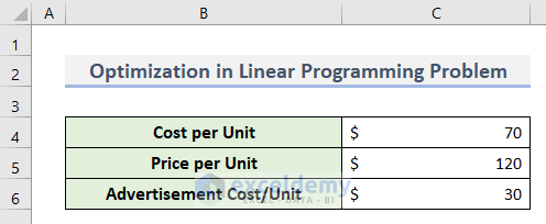
First, determine the values of Cost per Unit, Price per Unit and the Advertisement Cost per Unit for the specific product in the Cell range B5:C6.

Then, specify the Available No. of Units and the Budget for Advertisement for each publisher in the Cell range C9:D10.

Now, we will calculate some parameters for Publisher 1.
For this, insert this formula in Cell C11 to determine the Sold Number of Units.

=MIN(C10/C6,C9)

Here, we used the MIN function to get the minimum value.

Then, find out the Revenue in Cell C12 with this formula.

=C5*C11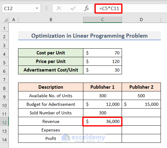

Following this, calculate Expenses in Cell C13 with this formula.

=C4*C9+C10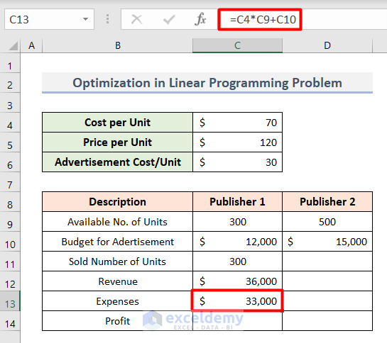

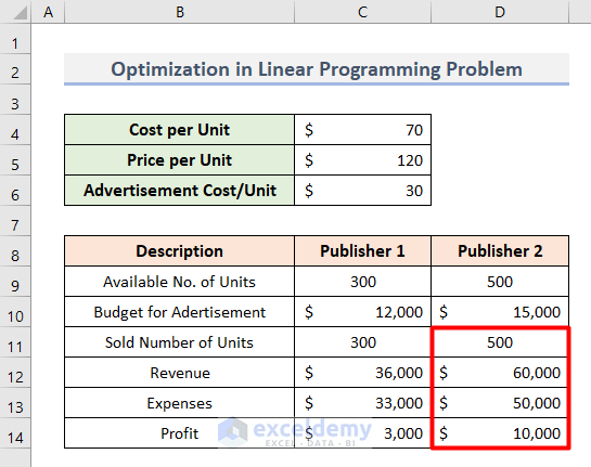
Lastly, apply this formula to calculate Profit in Cell C12.

=C12-C13

Along with it, apply the same process for Publisher 2 and get the following output.

Next, we will determine the constraints in separate cells.
To do this, count the total Budget for Advertisement with this formula and determine as Constraint 1 in Cells C16 and D16.

=C10+D10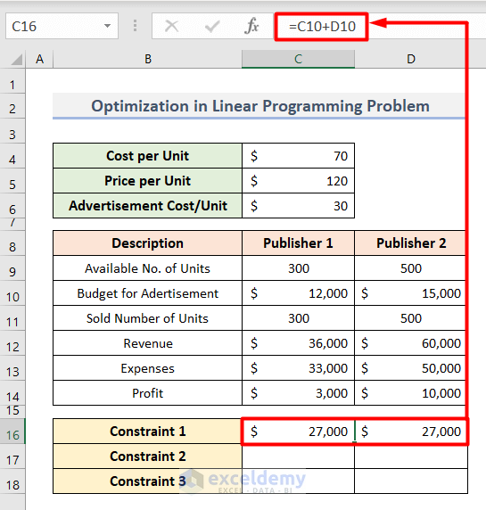

Then, use the following cell references as Constraint 2 for Publisher 1.
Type the formula below in Cell C17:

=C11

Also, type the following in Cell D17:

=C7

Lastly, we need to insert cell references as Constraint 3.

To do so, write the formula below in Cell C18:

=D11

Also, type the following in Cell D18:

=D7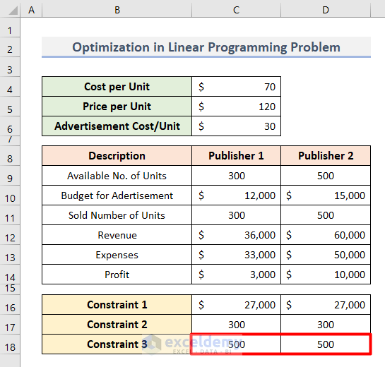

Alon with this, count the Total Profit in Cell C19 with this formula.

=C14+D14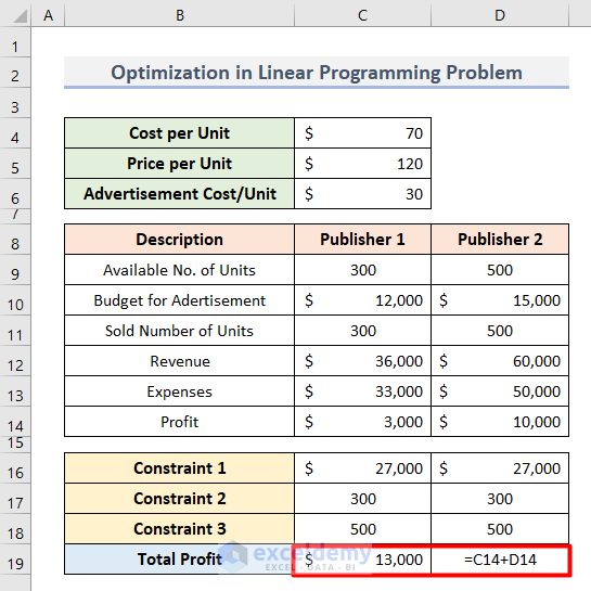

Up next, provide cell references in the Set Objective and By Changing Variable Cells in the Solver Parameters dialogue box.

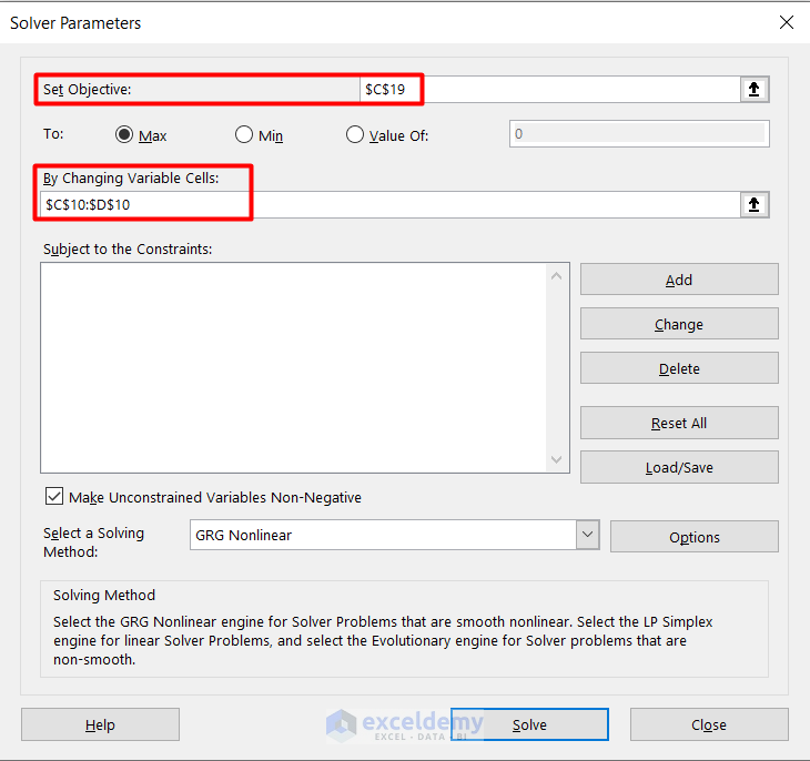
Then, insert the first Constraint and its relevant Cell Reference like this.

Afterward, keep adding new constraints by pressing Add in the Add Constraint window and click on OK when it is done.
Finally, you will see all the conditions in the Subject to the Constraints box.

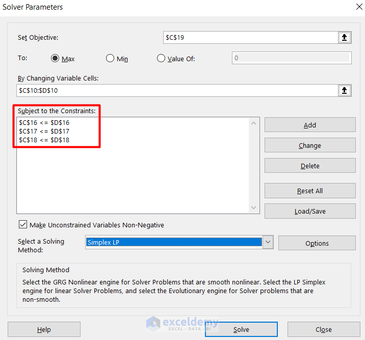
Along with this, select Simplex LP as the solving method.

Thereafter, press Solve.
That’s it, you will see that the Total Profit is optimized and the Budget for Advertisement also changed accordingly.

3. Nonlinear Problem Optimization with Constraints in Excel

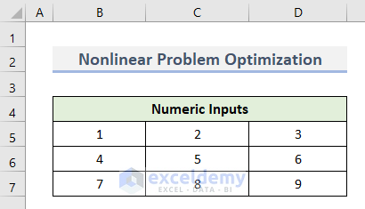
In this last case, we will consider the popular Magic Square puzzle where we will do optimization. Here, we need to calculate the horizontal, vertical and diagonal values which sum up to 15 which is the constraint. To do this, follow the steps below.

In the beginning, insert the numbers from 1 to 9 in the Cell range B5:D7 like this.

Then, count the total value of the first row with this formula in Cell E5.

=SUM(B5:D5)

Here, we used the SUM function to get the total value.

Afterward, use the AutoFill tool to calculate the Sum of Rows for Rows 2 and 3.

Next, calculate the Sum of Column for the 1st column with this formula.

=SUM(C5:C7)

Then, apply a similar process to the other 2 columns.

Lastly, calculate Diagonal Sum with this formula for left angle diagonal values.

=SUM(C5,D6,E7)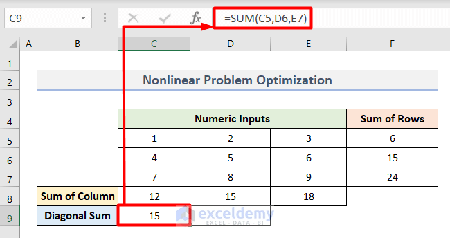

Similarly, count the same for right angle diagonal values.

=SUM(E5,D6,C7)

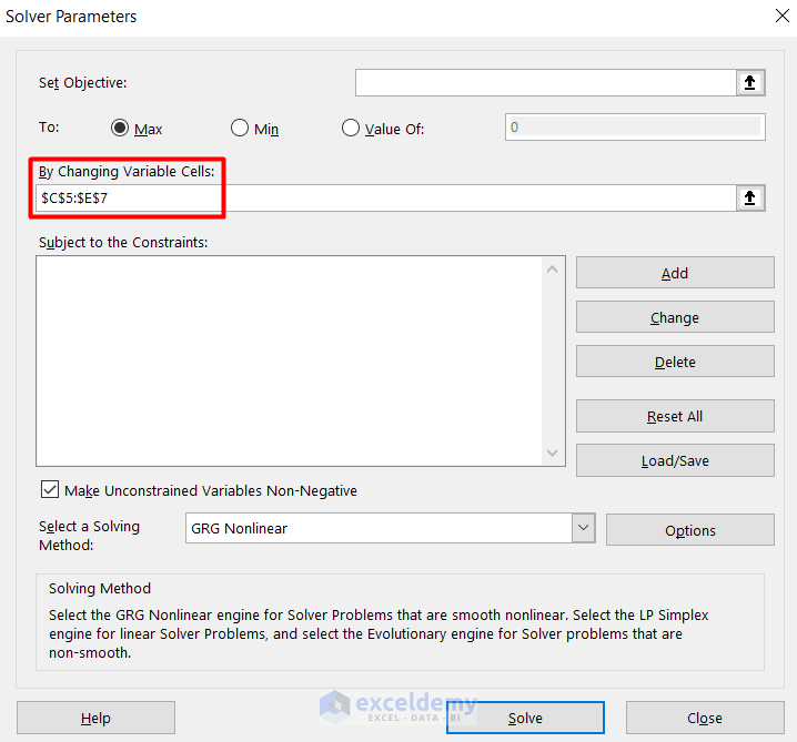
Next, open the Solver Parameters window and insert the Variable Cell reference.

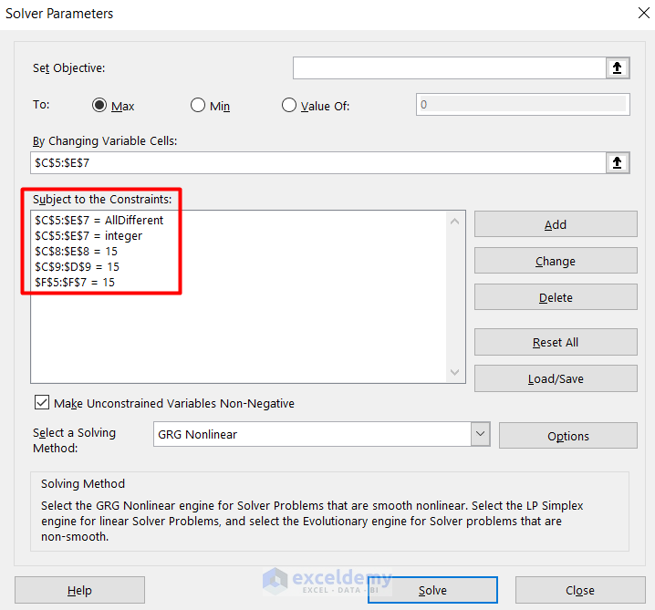
After this, provide the Constraints as shown below.

Thereafter, keep GRG Nonlinear as the solving method.

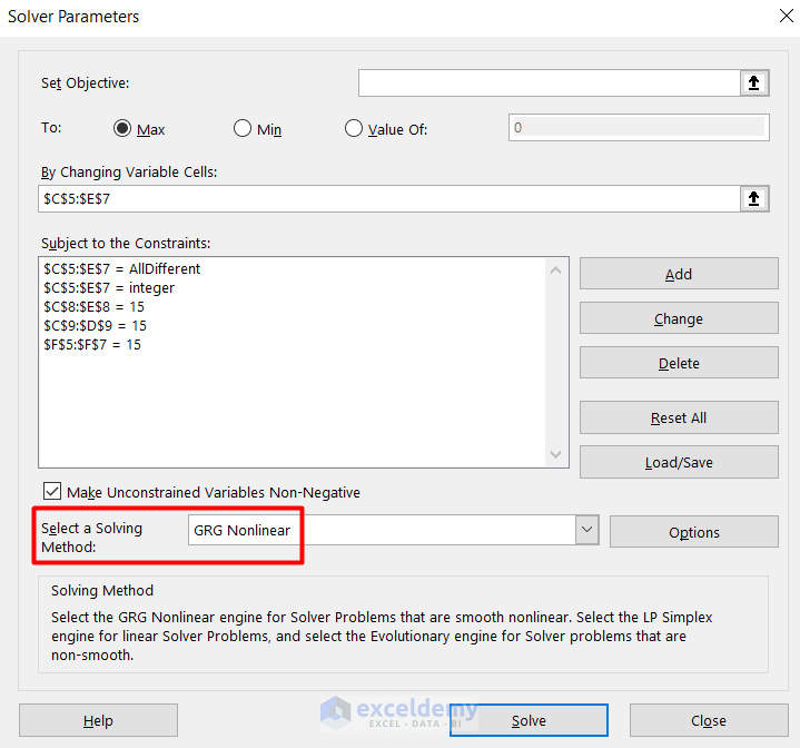
Lastly, press Solve.
As a result, you will notice that the values in Numeric Inputs are optimized and therefore their cumulative values are 15 on each side.

Conclusion

That’s all for today. Get the sample file to learn the process of Excel optimization with constraints through 3 case scenarios. Let us know your feedback in the comment box.

<< Go Back to Optimization in Excel | Solver in Excel | Learn Excel