In this article, we will learn about the syntax of DAX formulas for Power Pivot. We will also learn where to use DAX formulas and how to use DAX formulas for Power Pivot.
We can use the DAX formulas for Power Pivot in various business situations. You can apply formulas for sales analysis, inventory management, budgeting, and forecasting, etc.
When we need to find any row-wise data from the given columns (e.g. sales from the multiplication of unit price and quantity), more importantly, in the calculation area, we can determine a specific value based on single or multiple criteria using the Measures command.

Download Practice Workbook
You can download the practice file here.
Syntax of DAX Formulas
DAX (Data Analysis Expressions) is a formula language for Power Pivot and Power BI.
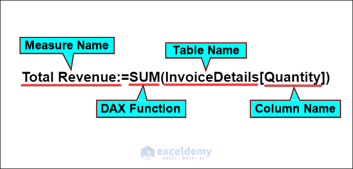
The DAX formula contains multiple components. These are:
- Measure Name: The name of the calculation. You can rename it according to your preferences.
- DAX Function: There are more than 250 DAX functions. You have to input the appropriate functions. Remember, there is a difference between Excel functions and DAX functions.
- Table Name: Sometimes, it will be in a single quote.
- Column Name: It will be in square brackets.
You can better understand the syntax from the following visual representation.
Where to Write DAX Formulas in Power Pivot
We can use DAX formulas in two different places in Power Pivot. We will discuss these in the following part of the article.
1. Calculated Column
A calculated column in Power Pivot is a column you can add to a table using Data Analysis Expressions (DAX) formulas. You can perform calculations based on the values in other columns of the same table or other related tables by using DAX formulas. Following that, the calculated values for each row in the table are placed in the calculated columns.
- First, click on the Add Column named column’s header.
- Then, in the formula bar, enter your formula. In the highlighted red box area.
- After that, press the Enter
- Finally, the formula result will appear in the calculated column.
2. Measures Command in Power Pivot
A measure in Excel’s Power Pivot is a DAX formula that computes an aggregate, calculation, or result based on a set of values.
- To start, select New Measure under Measures on the Power Pivot tab.

- After that, the Measure dialog box will appear.
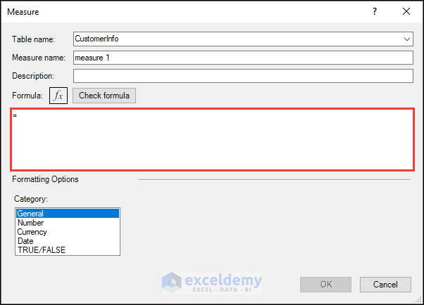
In the formula box, you can write the DAX formula. Some other things that you can specify (optional) Measure Name, description, etc. Another important thing is to choose the Table Name to apply the DAX formula.
- After writing the DAX formula, you have to press OK.
Prepare Data to Apply DAX Formulas for Power Pivot
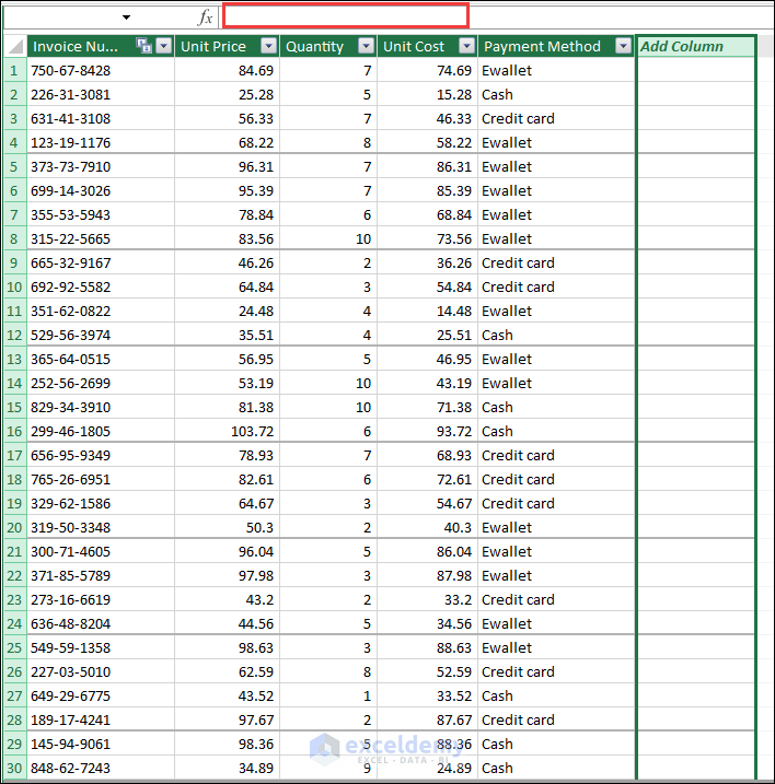
We will be using a workbook in Excel with three separate worksheets. These sheets contain data about “Customer Information”, “Invoice Log”, and “Invoice Details”. You must first prepare your dataset before using DAX in Power Pivot. Follow these steps:
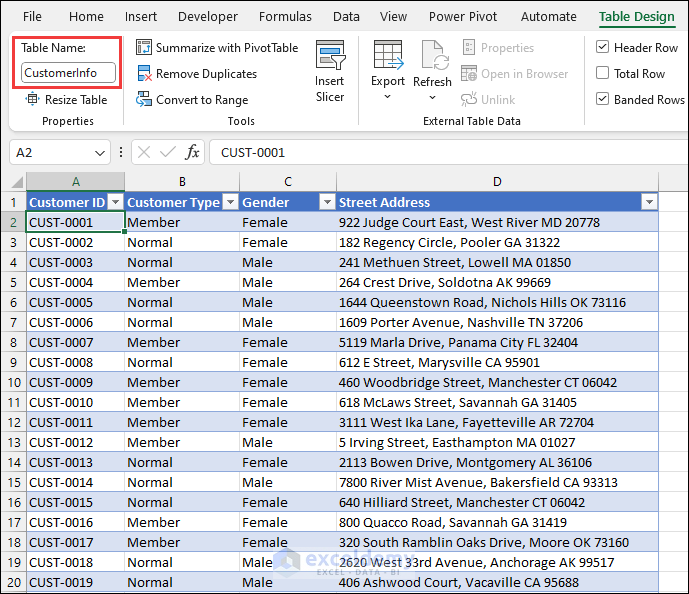
- First, we will convert the dataset from each sheet into a table.
- Now, you have to give each table a meaningful name so you can find it when writing DAX Click on Table Design and then edit the Table Name.
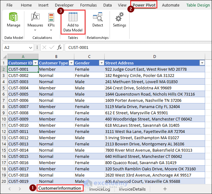
- Then, launch the Power Pivot’s Data Model and navigate to the sheet you want to include.
- Following that, select Add to Data Model from the Power Pivot tab.
- Next, follow the same steps to add the remaining tables to the data model.
- After that, go to the Power Pivot tab and choose the Manage option.

- Consequently, Excel’s Power Pivot interface will become visible.
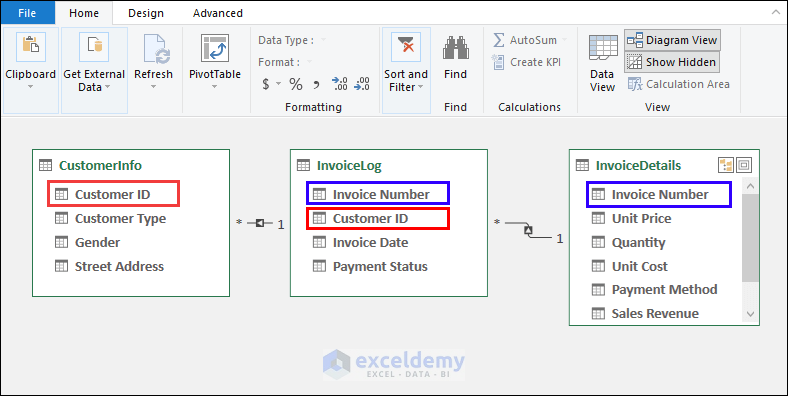
- Now, we will create a relationship between the tables. We can do that in the Diagram View.

- Following that, we will choose the name of the table’s field that you will use to establish a relationship with another table.
- Then, drag the field to the corresponding field in the second table.
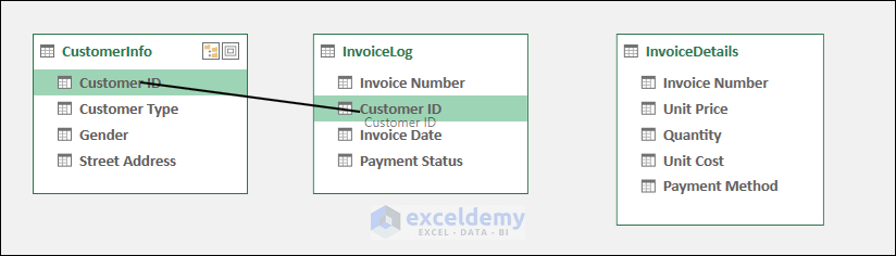
- After that, we can create the relationship between the tables “CustomerInfo” and “InvoiceLog” based on the common field CustomerID.
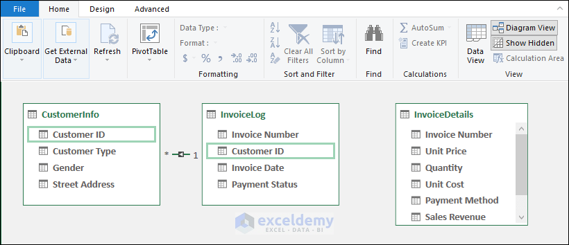
- Next, create all the relationships by dragging and joining the common headers.
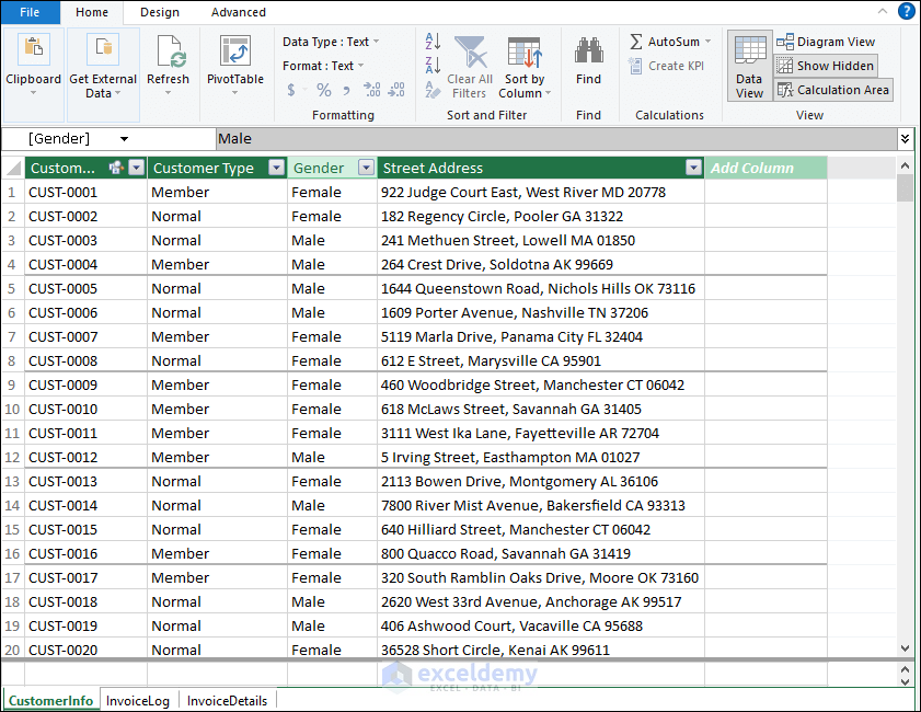
- Subsequently, click on the Data View if you have created the relationships.
- As a result, the Data View of the sheets will appear.

- You can now use DAX functions and formulas to get the value of the calculated field.
- Here, we will insert a formula in the calculated column of the InvoiceDetails table.
=Total Revenue:=InvoiceDetails[Quantity]*InvoiceDetails[Unit Cost]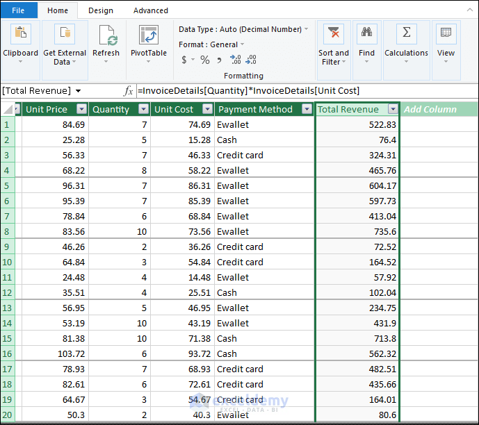
- This DAX formula will show all the order revenues in a new column.
How to Use DAX Formulas for Power Pivot: 5 Practical Examples
1. AVERAGE Function
The AVERAGE function calculates the average of a numeric column or expression in a table. It determines the total number of values in the chosen column and divides that total by the number of non-blank values.
Syntax:
AVERAGE(<column>)We can use the AVERAGE function in DAX to calculate average values from the dataset.
- First, select a cell outside the table.
- Next, insert the following formula in the table.
Average Sales Per Order:=AVERAGE(InvoiceDetails[Total Revenue])- As a result, we will see average sales per order.
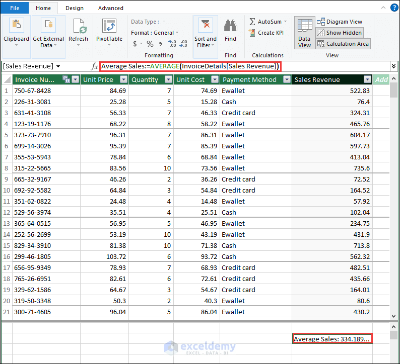
- If you notice, you will see that the result value contains infinite values after decimal.
- So, keep the cursor on the cell and right-click on the mouse.
- After that, it will show the Format option; click on that.
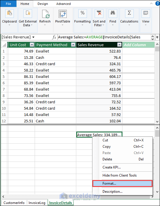
- Next, a dialog box will appear. Set the category to Number and set your desired decimal places.
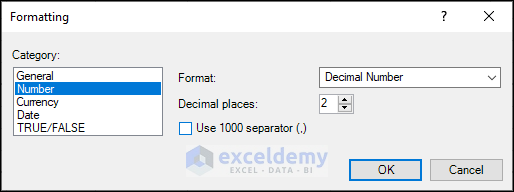
- Finally, it will change the decimal values of the result.
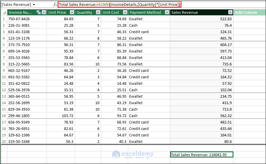
2. SUMX Function
The SUMX function in DAX is used to loop through a table and accumulate totals. It processes each row by evaluating an expression and adding up the values. It is useful when you need to run a calculation on each row of a table and then add up the results to get a grand total.
Syntax:
SUMX(table, expression)We need to multiply the Quantity and Unit Price of each order, then add the results to determine the “Total Sales Revenue”. The SUMX function in DAX is the only function that is suitable in this situation.
- First, select a cell and insert the following formula in the formula bar.
Total Sales Revenue:=SUMX(InvoiceDetails,[Quantity]*[Unit Price])- Then, the formula will return the Total Sales Revenue, counting all invoices.
3. CALCULATE Function
The CALCULATE function in DAX is one of the most useful and robust functions available. This is useful for changing the context in which a DAX expression is evaluated. This is particularly helpful for applying filters, altering the row context, and running conditional calculations.
Syntax:
CALCULATE(<expression>, <filter1>, <filter2>, ...)
In this dataset, we will calculate the total number of pending orders. Here, we will combine the CALCULATE function with the COUNTROWS function.
- First, select a cell and insert the following formula in the formula bar.
Total Pending Orders:=CALCULATE( COUNTROWS(InvoiceLog), InvoiceLog[Payment Status] = "Pending" )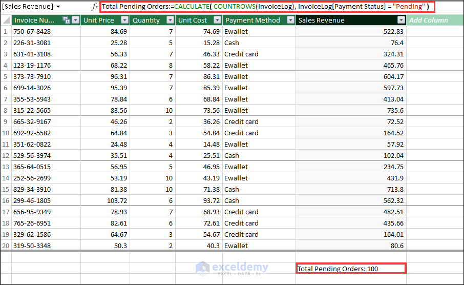
Formula Breakdown
- COUNTROWS(InvoiceLog): This formula counts the number of rows in the “InvoiceLog” It gives you the total number of orders, regardless of payment status.
- InvoiceLog[Payment Status] = “Pending”: This is a filter condition. It restricts the calculation to include rows where the “Payment Status” column has the value “Pending”.
- CALCULATE( COUNTROWS(InvoiceLog), InvoiceLog[Payment Status] = “Pending” ): This function allows you to modify the filter context of a calculation. It takes an expression as its first argument and optional filter conditions as subsequent arguments.
4. FILTER Function
The FILTER function in DAX filters data taken from a table based on a predetermined set of conditions that the user specifies. It will return a table that contains only those rows in the table that meet the criteria that you provide.
Syntax:
FILTER(Table, Condition)I only want the sales for quantities under “5” to be calculated in my dataset. In this instance, I will combine the SUMX function and the FILTER function.
- In the beginning, select a cell where you want to see the result.
- Then, insert the following formula in the formula bar.
Total Sales for Quantity<5:=SUMX(FILTER(InvoiceDetails,[Quantity]<5),InvoiceDetails[Quantity]*InvoiceDetails[Unit Price])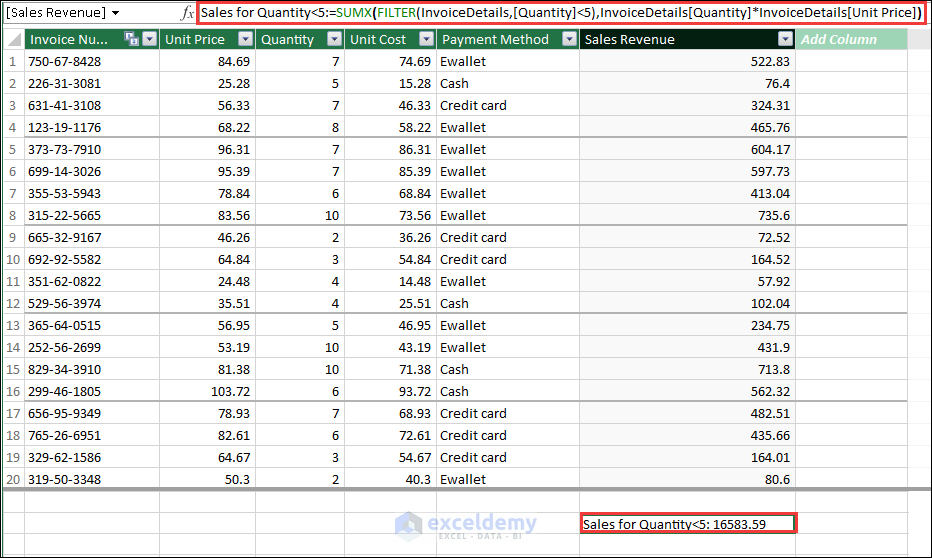
Formula Breakdown
- FILTER(InvoiceDetails, [Quantity] < 5): This function filters the InvoiceDetails table to include only the rows where the quantity is less than 5.
- SUMX(FILTER(InvoiceDetails,[Quantity]<5), InvoiceDetails[Quantity]*InvoiceDetails[Unit Price]): This part calculates the sum of the product of quantity and unit price for each row in the filtered table from step 1. SUMX loops through the filtered table, multiplies each row’s quantity by its unit price, and then adds up the totals.
5. IF Function
The IF function in DAX checks if a condition is true or false and returns a different value depending on the result.
Syntax:
IF(LogicalTest, ValueIfTrue, ValueIfFalse)We will use the IF function to determine which orders are retail and which are bulk orders.
- First, we select a new column and insert the following formula.
=IF(InvoiceDetails[Quantity] >= 10, "Bulk", "Retail")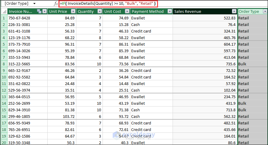
- As a result, it will return the result in the rows of that particular column.
Things to Remember
- It is very important to set up the right relationship between the tables. Unexpected outcomes can result from missing or incorrect relationships.
- In your DAX formulas, always double-check the names of the columns and tables. Errors will occur if the name of the data model and the formula inputs are different.
Frequently Asked Questions
1. How to use the DAX function in Power Query?
Power Query does not directly use DAX functions. Power Query shapes and transforms data using the ” M ” programming language. While Power Query handles data preparation and transformation before the data is loaded into the model, DAX is typically used in measures and calculated columns within the data model.
2. What is the use of the Related () DAX function?
The `RELATED()` DAX function retrieves values from a related table in a one-to-many or many-to-one relationship within a data model.
3. Is there any difference between Calculated Columns and Measures?
Measures and Calculated Columns differ in a number of specific ways. Calculated columns are performed while data is being loaded or refreshed. Once the calculations are completed, a new column is added to the table with the results. However, Measures are specifically made for aggregating data and performing calculations that involve summarizing it, such as sums, averages, counts, ratios, etc.
Conclusion
In this article, we discussed the syntax of DAX formulas in Excel. We also discussed where and how to use DAX formulas for Power Pivot in Excel. We sincerely hope you enjoyed and learned a lot from this article. Additionally, if you want to read more articles on Excel, you may visit our website, Exceldemy. If you have any questions, comments, or recommendations, kindly leave them in the comment section below.
<< Go Back to DAX in Power Pivot | Power Pivot Excel | Learn Excel

