In this Excel tutorial, you will learn 2 useful examples of calculating percentage with criteria. We will discuss how to use the IF function to calculate percentage with criteria in Excel. And then another advanced-level example where we will calculate the percentage of cells with a specific color in Excel.
Calculating percentages with criteria is commonly used in scenarios involving data analysis or financial modeling. For instance, you may need to determine the percentage of sales that meet a specific condition, such as products with sales exceeding a certain threshold. We can utilize functions like IF, COUNTIF, COUNTA, SUMIF, etc. to calculate percentages with criteria in Excel. Now let’s delve into the examples.
How to Use IF Function to Calculate Percentage with Criteria in Excel
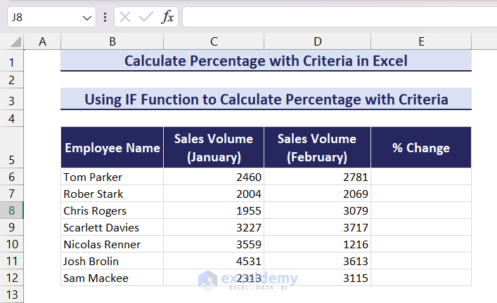
Consider the following dataset where we have the sales volume of some employees for two consecutive months. We want to calculate the percentage of change in sales volume. However, if the change in sales volume is negative, we will assign the word “Decrease” instead of calculating the percentage change for that employee. To do this, we can apply the IF function.
In cell E6, apply the following formula and press the Enter key=> set the Number Format of the cell to Percentage => drag down the Fill Handle icon to copy the formula in the remaining cells.
=IF(D6-C6>0,(D6-C6)/C6,"Decreased")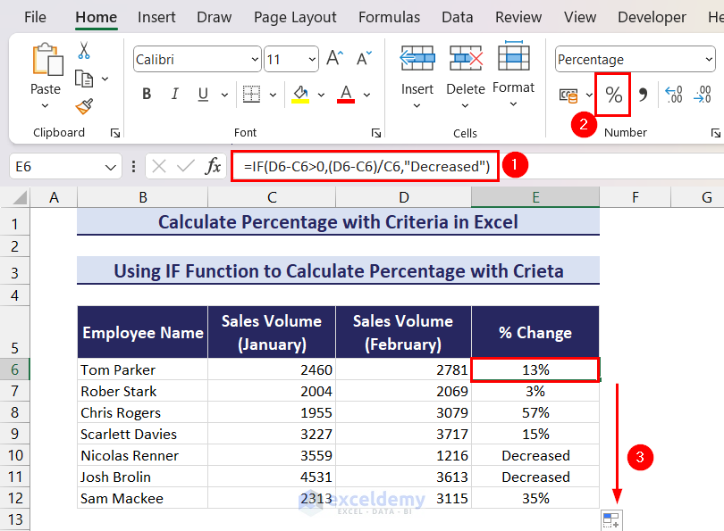
How to Calculating Percentage Based on Cell Color in Excel
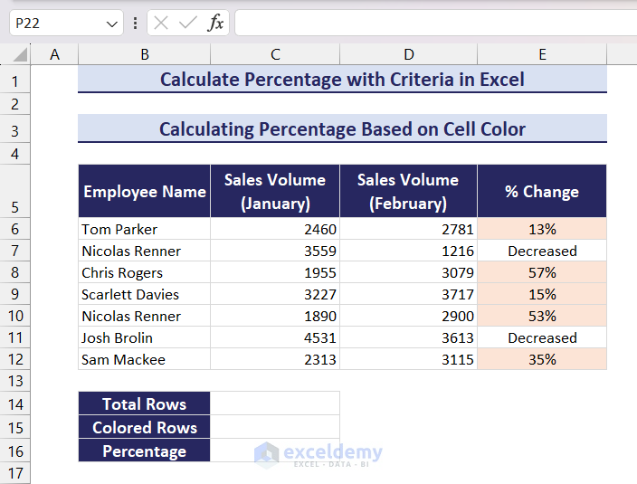
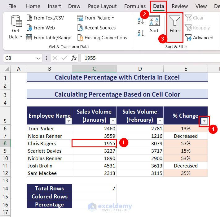
Now, look at the following dataset. We have set colors for the cells that have a positive percentage change value and the cells with the word “Decreased” are ignored. (You can achieve this manually or by using Conditional Formatting). We want to calculate the percentage of rows that have this color criteria.
First, in cell C14, apply the following formula and press the Enter key to count total rows.
=COUNTA(E6:E12)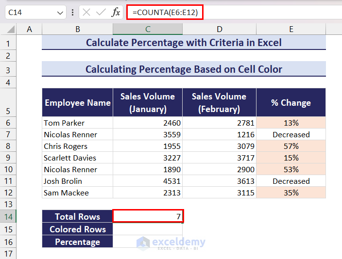
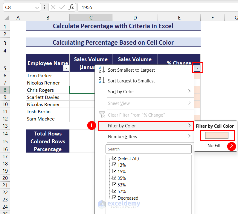
Afterward, select any cell in the dataset => go to the Data tab and click on the Filter button => When the filter dropdown icons are visible, click on the dropdown icon of the column where you want to apply the color criteria filter.
In the dropdown menu, click on the Filter by Color option and then select the desired cell color.
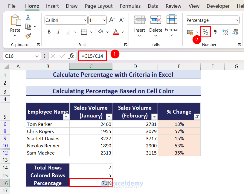
Now, only the rows that contain colored cells are visible. To calculate the count of only visible rows, we can apply the SUBTOTAL function. Apply the following formula in cell C15 and press the Enter key.
=SUBTOTAL(3,E6:E12)
Finally, apply the following formula in cell C16 and set the Number Format to percentage.
=C15/C14Now, you will have your desired output.
This concludes our article on how to calculate percentage with criteria in Excel. We discussed two useful examples: using the IF function to calculate the percentage with criteria and determining the percentage of rows based on cell color criteria in Excel. We hope this article will be helpful for you. Let us know your feedback in the comment section.
Calculate Percentage with Criteria in Excel: Knowledge Hub
<<Go Back to Calculating Percentages in Excel | How to Calculate in Excel | Learn Excel

