In some cases, we need to filter the Pivot Table to get our desired output. Luckily, there are many effective methods to do that task. In this article, I’ll discuss the 8 most effective and popular methods to filter Pivot Table in Excel with proper explanation.
As the article will be a little bit lengthy. You may look over the contents to choose the suitable one based on your preference. For your convenience, I’ll cover the easiest example first, then the filtering methods for multiple columns, and lastly a VBA method.
How to Filter Excel Pivot Table: 8 Effective Methods
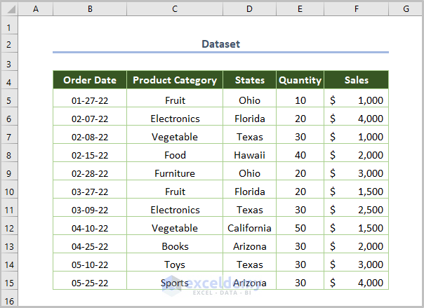
This is our dataset where the Product Category is given with their Order Date, Quantity, Sales based on the States of the U.S.
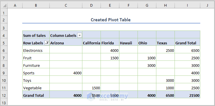
I created a Pivot Table which is as follows.
Let’s dive into the methods of filtering the Pivot Table.
1. Using Report Filter to Filter Excel Pivot Table
Firstly, we’ll use the Report Filter to screen the information in the Pivot Table.
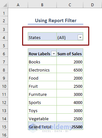
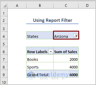
For example, we want to get the sum of sales for all product categories in Arizona state.
Now, follow the steps below.
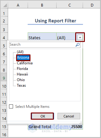
⏩ To turn on Report Filter, select the States field and drag down the field into the Filters areas.
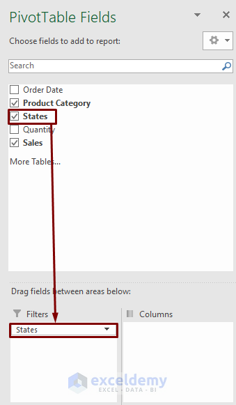
⏩ Then, you’ll see a drop-down arrow with the field States.
⏩ If you click on the drop-down arrow, you’ll get all states in the filtering option.
Select the Arizona option and press OK.
⏩ So, the following output is the desired output that you wanted to get.
2. Utilizing Value Filters
When you need to filter based on value, Value Filters will be a better choice to get such results. More importantly, there are numerous filtering options inside Value Filters. Off them, we’ll see three notable ways of filtering depending on values.
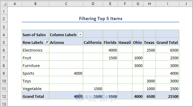
2.1. Value Filters to Get Top Items
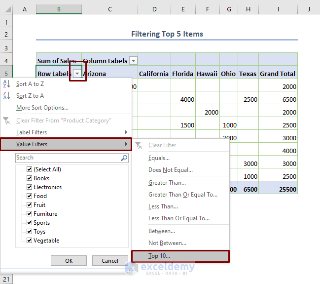
For instance, you have to filter the top 5 items on the basis of the sum of sales.
⏩ Click on the drop-down arrow of Row Labels.
⏩ Go to Value Filters > Top 10.
⏩ Input 5 instead of 10 and press OK.
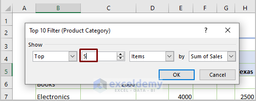
This is the expected output.
2.2. Value Filters to Return
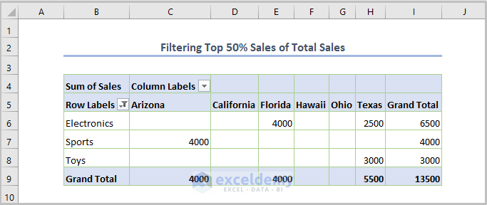
Say, you want to filter the top 50% sum of sales from the total sum of sales.
For finding out this, just go on the Top 10 Filter option likewise the previous example.
⏩ And input 50 instead of 10 and choose Percent, and lastly press OK.
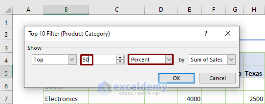
⏩ So, the following product has the top 50% sales of total sales.
2.3. Value Filters for a Specific Value
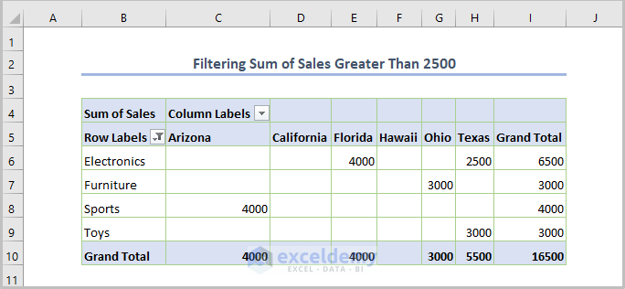
Furthermore, you can filter the whole Pivot Table by specifying a value. Suppose, you want to get the sum of sales that is greater than 2500.
⏩ Click on the drop-down arrow of Row Labels.
⏩ Go to Value Filters > Greater Than.

⏩ And now, put the specified value in the box that is 2500 and press OK.
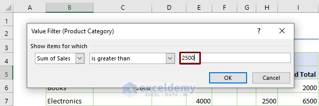
⏩ Immediately, you’ll get the following output where all the sum of sales is greater than 2500.
3. Applying Label Filters to Filter Excel Pivot Table
While dealing with the Value Filters, you might observe an option i.e. Label Filters.
Well, now, we’ll explore its usage.
Assuming that you want to filter the product category that contains Books only.
I mean you want to find the sum of sales for the Books.
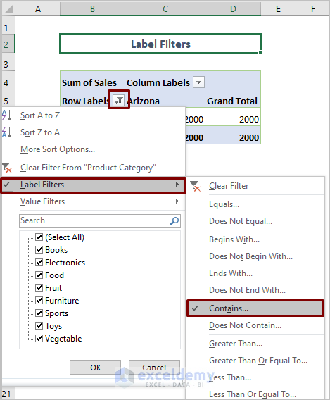
⏩ Click on the drop-down arrow of Row Labels.
⏩ Go to Label Filters > Contains.
⏩ Type the word Books in the desired option of the Label Filter dialog box.
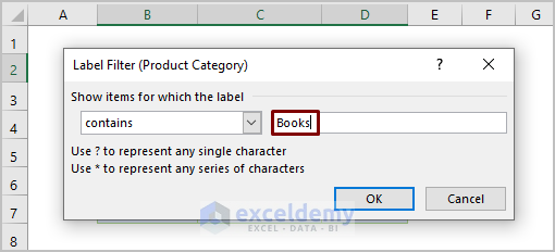
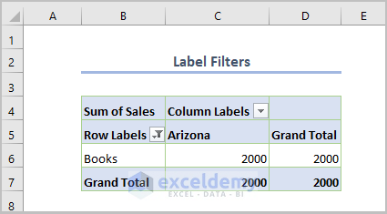
⏩ After pressing OK, you’ll get the filtered Pivot Table on the basis of Books.
4. Creating Date Filters
Now, we’ll see another filtering method that is for separating the Pivot Table depending on the dates.
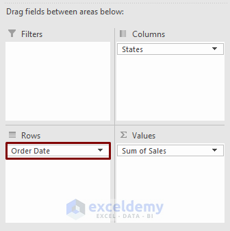
As you already know, we have a field namely Order Date.
And if you want to filter the Pivot Table for a specific date range e.g. 02-15-22 to 5-10-22.
⏩ For doing this, drag the Order Date field inside the Rows areas.
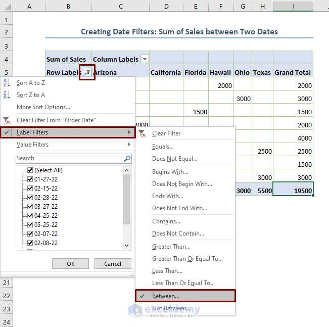
⏩ Then go to Label Filters > Between.
⏩ Fix the desired dates in the following Label Filter dialog box.
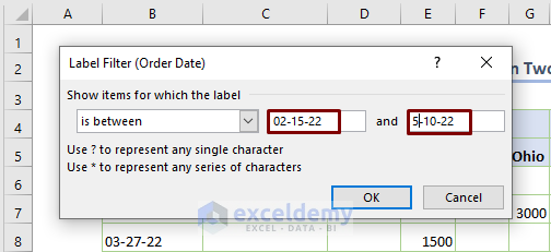
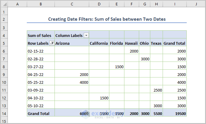
⏩ While entering the OK option, you’ll get the following output.
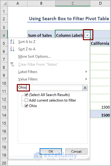
5. Using Search Box to Filter Excel Pivot Table
Using Search Box is really a simple method. Just type the word (e.g. Ohio as shown in the following figure) that you want to filter the Pivot Table.
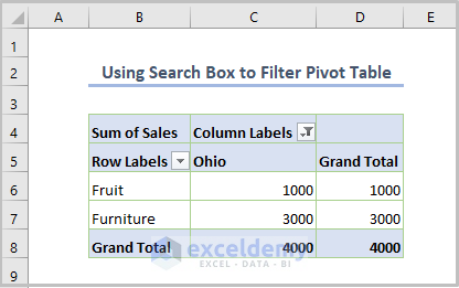
So, the following output is the filtered Pivot Table containing the state Ohio.
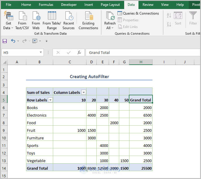
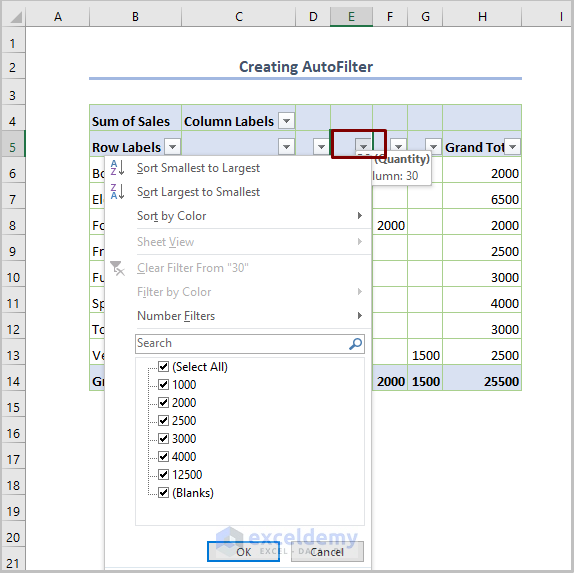
6. Using AutoFilter to Screen Pivot Table
If you’re not a new user in Excel, you must have heard the name of the Filter option. Unfortunately, the Filter option is not working for the Pivot Table as shown in the following figure.
But when I keep the cursor over an adjacent cell of the Pivot Table, the Filter option is working.
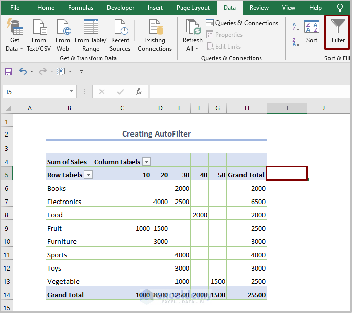
After clicking on the Filter option, you’ll see surprising drop-down arrows for all columns. Now, you can filter any column without following other methods.
7. Method to Filter Multiple Items in Excel Pivot Table
The most sophisticated and popular method of filtering the Pivot Table in Excel is to filter multiple columns. Obviously, it’ll save you time and you can filter on the basis of your requirements quickly.
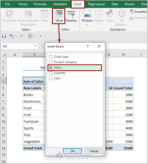
7.1. Filter Multiple Items Using Slicer
We can filter the Pivot Table on the basis of States in a faster way by using Slicer.
Select a cell within the Pivot Table
⏩ Go to Insert tab > Slicer from the Filters ribbon
⏩ Choose the States while watching the Insert Slicer dialog box.
⏩ Now, you see a moveable filtering option of States (the right side of the following picture).
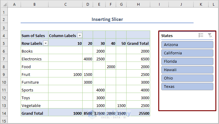
So, you may have a question about how it works.
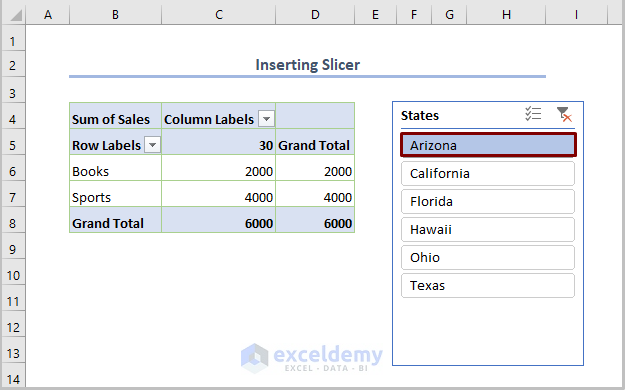
Just select a state e.g. Arizona from the options as depicted in the following figure. And you’ll get the output instantly at the Pivot Table located on the left side of the figure.
7.2. Filter Multiple Items Using Comma
Furthermore, if you want to display the filter criteria in a single cell, you can do that using the TEXTJOIN function.
For example, if you input the following formula in the G4 cell.
=TEXTJOIN(",",TRUE,B6:B15)Here, “,” is the delimiter, TRUE for ignoring empty cells, B6:B15 is the cell range for the Product Category of the dataset.
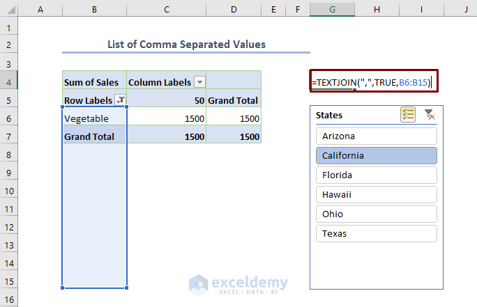
After entering the formula, we’ll get the filtering criteria in a single cell whatever we want to filter by selecting in the Slicer.
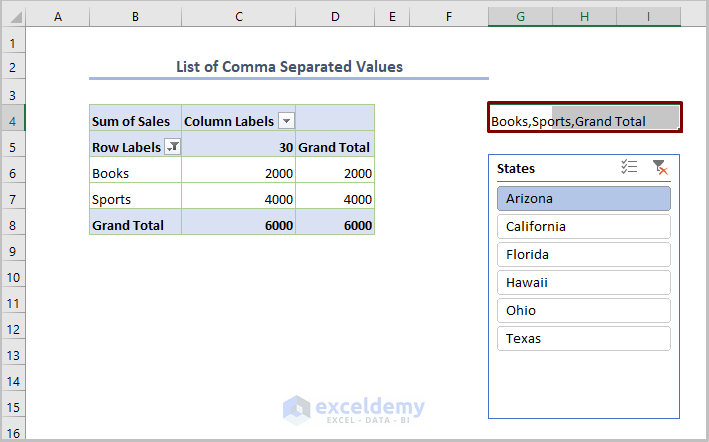
Here, the filtering criteria i.e. Books, Sports are seen in the G4 cell.
7.3. Filter Multiple Items Using Filter Criteria
In this way of filtering multiple items, I’ll show you how to join two Pivot Tables and apply filtering together for the two tables.
Regarding this, we have to copy the Pivot Table by pressing CTRL + C and paste the table at a close location of the existing table by pressing CTRL + V.
The below image depicts the process.
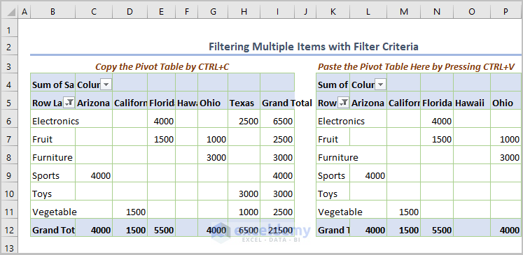
After doing that, keep the Row Labels only in the case of the second Pivot Table.
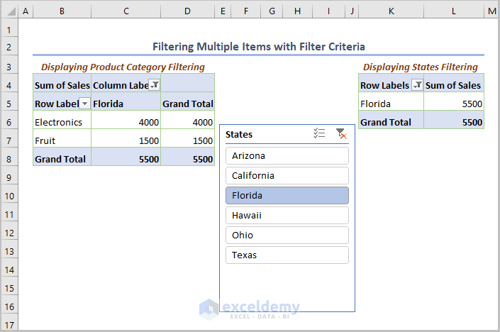
Now, if you choose any state (e.g. Florida) from the Slicer, the filtering method will work for two Pivot Tables simultaneously.
The first Pivot Table filters product categories whereas the second table filters on the basis of States.
So what’s the fact behind this filtering?
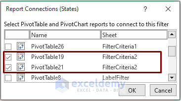
Right-click on the Slicer, and select the Report Connections option.
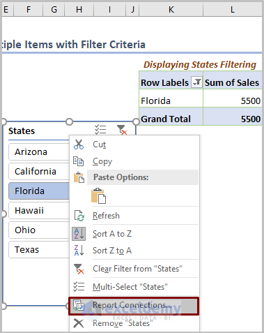
You’ll get the following figure. The figure demonstrates that PivotTable19 (the first table) & PivotTable21(the second table) are joined.
8. Excel Pivot Table Filter Based on a Cell Value Using VBA
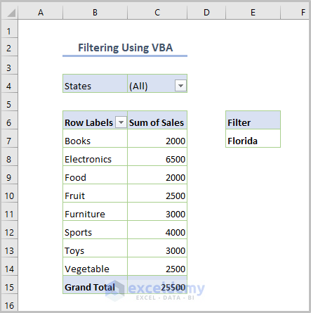
Lastly, I’m going to discuss a case, if you want to filter the Pivot Table for a specific cell value.
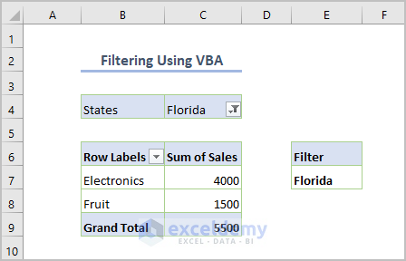
Let’s examine that you want to filter the whole Pivot Table on the basis of the state of Florida (located at the E7 cell).
Now follow the steps below.
Step 1:
As we want to use VBA, we must know how to insert a VBA code.
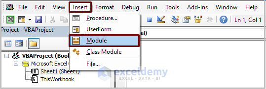
Firstly, open a module by clicking Developer > Visual Basic.
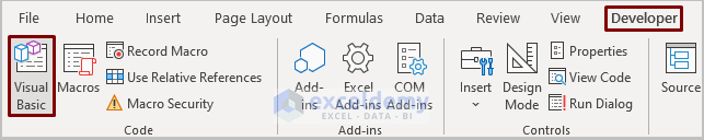
Secondly, go to Insert>Module.
Step 2:
Now copy the following code into your module.
Sub Filter_UsingVBA()
   Dim pvFld As PivotField
   Dim strFilter As String
   Set pvFld = ActiveSheet.PivotTables("PivotTable23").PivotFields("States")
   strFilter = ActiveWorkbook.Sheets("Sheet14").Range("E7").Value
   pvFld.CurrentPage = strFilter
End Sub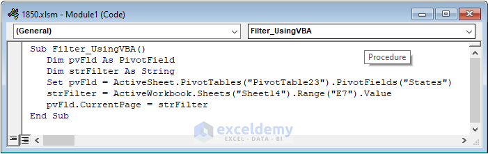
In the above code, I declared pvFld as PivotField and strFilter as String type. Then the required source for pvFld and strFilter are fixed.
Three basic things in the code are-
- Pivot Table Name: PivotTable23
- Field Name of the Table: States
- Active Sheet Name: Sheet14
- Location of Filter Value: E7 cell.
Step 3:
Next, run the code (the keyboard shortcut is F5 or Fn+F5). And you’ll get the filtered output.
Download Practice Workbook
Conclusion
In the above article, I tried to cover the methods for filtering the Pivot Table in Excel. I strongly believe that this article will articulate your Excel journey. However, if you have any queries or suggestions, please let me know in the comments section below.
How to Filter Excel Pivot Table: Knowledge Hub
<< Go Back to Pivot Table in Excel | Learn Excel

