In this Excel tutorial, you will learn to create a table of contents in Excel manually and automatically. We will use the Insert Hyperlink dialog box, Mouse Cursor, HYPERLINK function, and Developer Button to create a table of contents manually. Also, we can use Power Query and VBA Macro to make a table of contents automatically. Further, we’ll apply the Named Range to develop a dynamic table of contents.
Note: We have used Microsoft 365 to prepare this tutorial. However, the following operations are applicable in older Excel versions from Excel 2007.
It’s bothering to find a sheet when a workbook contains a bunch of sheets. On the other hand, we can jump to a specific worksheet from the table of contents with only one click.
What Is Table of Contents in Excel
The table of contents in Excel is the checklist or series that shows the sequence of worksheets. Sometimes it can be a sequence of workbooks or some defined tasks.
Some purposes of a table of contents are outlined as follows:
- It is almost impossible for any organization to work on a single sheet. As a result, multiple worksheets are required. Dealing with countless sheets in a workbook is a challenging task. Therefore, creating a table of contents in Excel is necessary.
- It makes the workbook look more organized and professional.
- Since it has keywords regarding the worksheet’s topics and sub-topics, a table of contents can make the workbook more searchable.
How to Create Table of Contents Manually in Excel
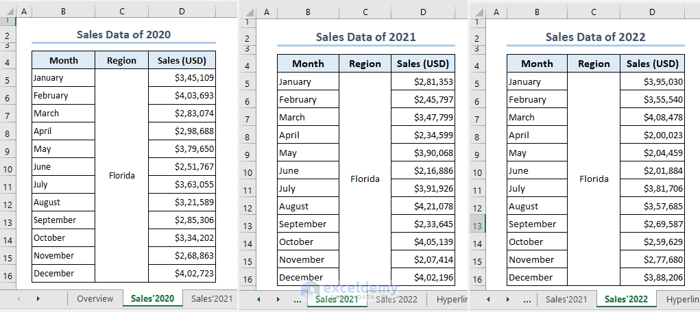
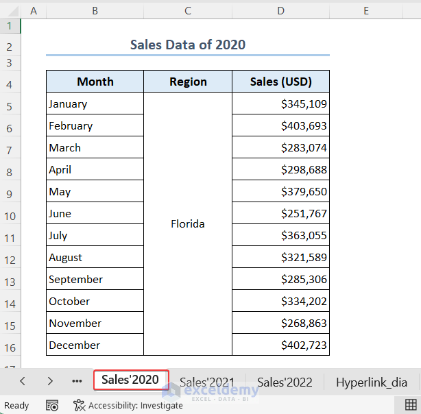
As you can see in the image, we are considering datasets containing 3 worksheets named Sales’2020, Sales’2021, and Sales’2022. You can use 4 approaches to create a table of contents manually in Excel. They are the Insert Hyperlink dialog box, HYPERLINK function, Mouse cursor, and Macro Button. Manually means, we’ll have to add each sheet individually in the table of contents.
Click for a detailed view
1. Using Insert Link Feature
The use of the Insert Hyperlink dialog box is the most convenient way to create a table of contents. You can simply get the dialog box from the Context menu list. Also, there are two other ways, keyboard shortcut and Insert tab.
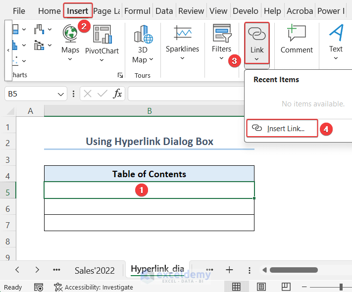
- First, select the B5 cell >> Right-Click on the Mouse >> Link >> Insert Link.

- Thus, the Insert Hyperlink dialog box appears. Alternatively, you can open the Insert Hyperlink dialog box by pressing the Ctrl + K Or, simply select the cell and click as follows: Insert >> Link >> Insert Link.
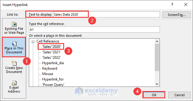
- Now, go to the Place in This Document >> Insert Sales Data 2020 in the Text to display >> Select the sheet Sales’2020 >> OK.
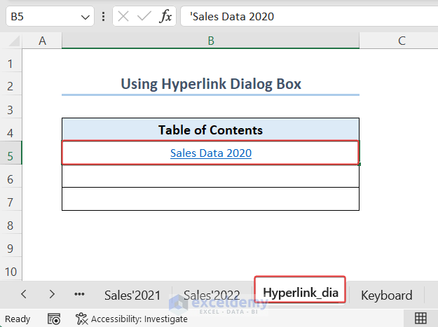
- Therefore, Sales Data 2020 appears in the B5 cell with a hyperlink.
- By clicking it, it will jump to the Sales’2020 worksheet.
- Similarly, we can insert the Sales Data 2021 and Sales Data 2022 in the table of contents with hyperlinks in B6 and B7 cells respectively.
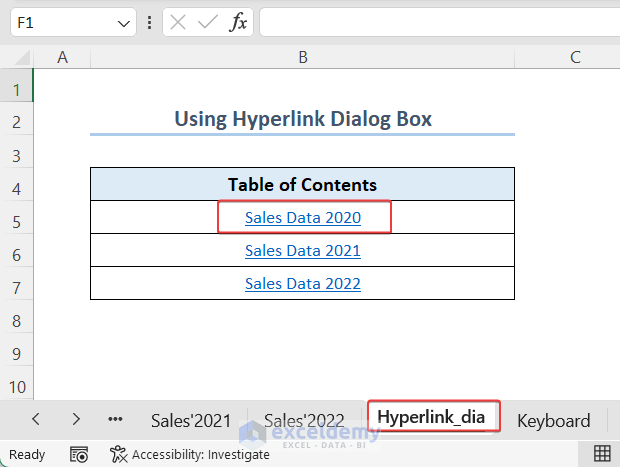
- Finally, we explore the Sales Data 2020 sheet by clicking on the B5 cell.
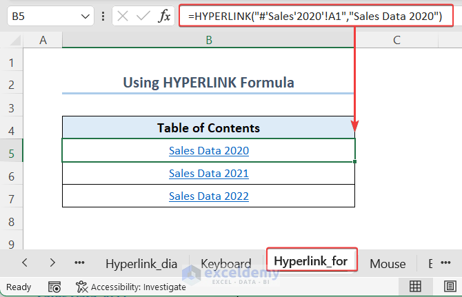
2. Apply HYPERLINK Function
We can use the HYPERLINK function to create hyperlinks manually. We can easily add hyperlinks to a table of contents using this suitable function within a minute.
- Applying the following formula in the B5 cell, you will be able to get a table of contents with hyperlinks.
=HYPERLINK("#'Sales'2020'!A1","Sales Data 2020")- From the formula of B5 cell, # dictates to remain in the current workbook. Sales’2020′!A1 is the location of the sheet. Sales Data 2020 is the text that is displayed in the cell.
Read More: Create Table of Contents with Hyperlinks
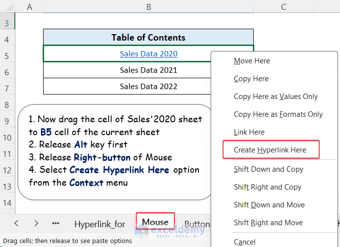
3. Using Mouse and Keyboard Shortcut
We can use the Mouse and keyboard shortcut to generate a table of contents including hyperlinks. You must be careful about the steps when you are applying this method.
- Selecting a cell and keeping the Mouse Cursor on the cell borderline >> Right-Click on the Mouse and hold >> Hold the Alt key.
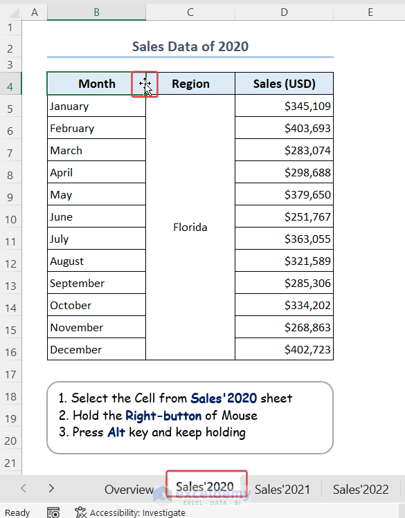
- After that, holding the Alt key and right-click together drag the Mouse to B5 of the current sheet.
- Later, release the Alt key >> Release the Right-Button of the Mouse >> A Context menu appears.
- Further, select Create Hyperlink Here from the Context Thus, we will be able to insert hyperlinks in the table of contents.
For better understanding please check out the video as follows:
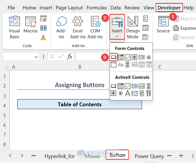
4. Assigning Macro Buttons for Sheets
You can assign a Button command from the Insert drop-down from the Developer tab. Also, you can say this is a macro-based approach since you must assign a VBA code to the Button.
- Initially, we prepared the below VBA code to jump to Sales’2020, Sales’2021, and Sales’2022 worksheets.
Sub Jump_to_Sales_2020()
ThisWorkbook.Sheets("Sales'2020").Activate
End Sub
Sub Jump_to_Sales_2021()
ThisWorkbook.Sheets("Sales'2021").Activate
End Sub
Sub Jump_to_Sales_2022()
ThisWorkbook.Sheets("Sales'2022").Activate
End Sub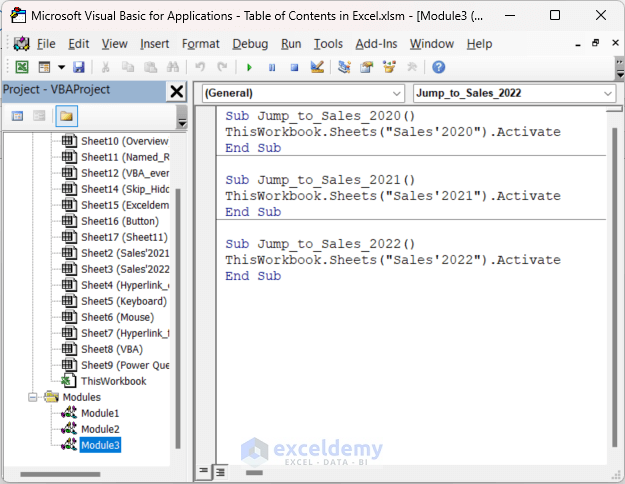
- Then click as follows, Developer >> Insert >> Button.
- Next, drag the to get the shape of the button.
- Consequently, the Assign Macro dialog box shows up. Then select Jump_to_Sales_2020 macro >> OK command.
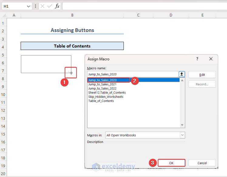
- Therefore, we obtain the Sales’2020 button by renaming it.

- Similarly, we create Sales’2021 and Sales’2022 button.
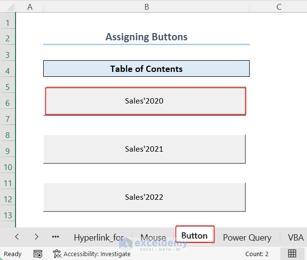
- You can jump directly to the Sales’2020 worksheet once you click the Sales’2020 button.

How to Make Table of Contents Automatically in Excel
Creating a table of contents Automatically is quite fascinating. Automatically means, all the sheets will be added to the table of contents at a time. Though you may find these tools a little bit complex, we will explain the applications concisely in this section. The 2 approaches are Power Query and the VBA Macro tool.
1. Using Power Query
Using the Power Query tool, you can automatically generate a table of contents. But you need to insert the HYPERLINK function to jump directly to the worksheet.
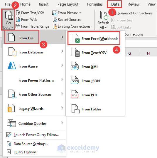
- To apply this method, go to the Data >> Get Data >> From Excel Workbook.
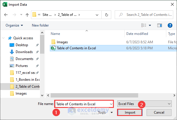
- Thus, a dialog box named Import Data shows up.
- Then, select Table of Contents in Excel file >> Import.
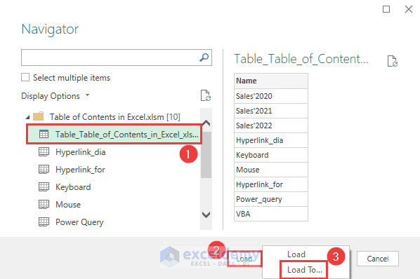
- After that, another dialog box named the Navigator dialog box.
- Select the Excel file from the Display Options field >> Load >> Load To.
- Further, fix the location B2 of the Power Query sheet by selecting the Existing worksheet from the Import Data dialog, and hitting the OK command.
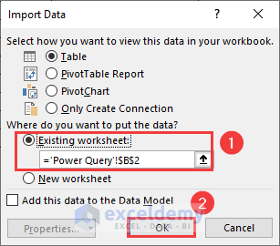
- Therefore, all table of content appears in the B2:B11 range automatically.
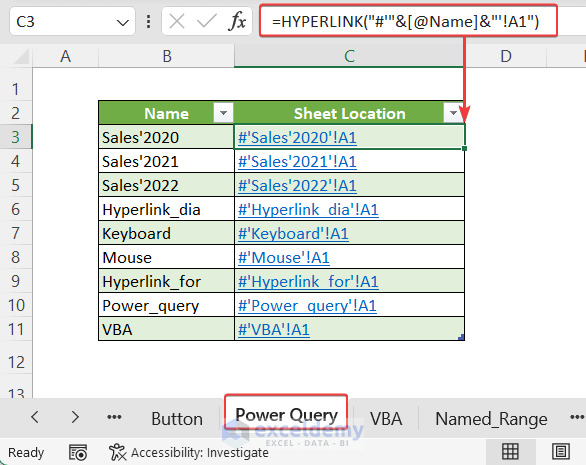
- Now it’s time to link them with the sheet so that we can jump within a moment.
- By inserting the following formula with the HYPERLINK function in the C3 cell, we automatically get a set of links in the C3:C11 range.
=HYPERLINK("#'"&[@Name]&"'!A1")
From the formula, # allows you to remain in the current workbook, [@Name] picks up the worksheet names and A1 is the cell of the worksheet. The Ampersand (&) operator bridges between texts.
2. Applying VBA Code
We can apply a simple VBA code that will allow you to get the table of contents automatically. In a large dataset containing numerous worksheets, it plays a vital role in developing a table of contents. You need to click the Run command every time to execute the VBA code and add a new sheet.
- Initially, go to the Developer >> Visual Basic. You must enable the Developer tab if the tab is not visible.
- Then from the VBA dialog box, select As follows: Insert >> Module.
- Next, insert the following codes in the Module and run by clicking the play icon or pressing the F5 key.
Sub Table_of_contents()
Set ws = Worksheets("VBA")
i = 1
Cells(2, 2).Value = "Table of contents"
For Each Sheet In ThisWorkbook.Sheets
            If Sheets.Count <> 0 Then
            i = i + 1
            ws.Hyperlinks.Add Cells(i + 1, 2), "", "'" & Sheet.Name & "'!A1", , Sheet.Name
            End If
Next
End Sub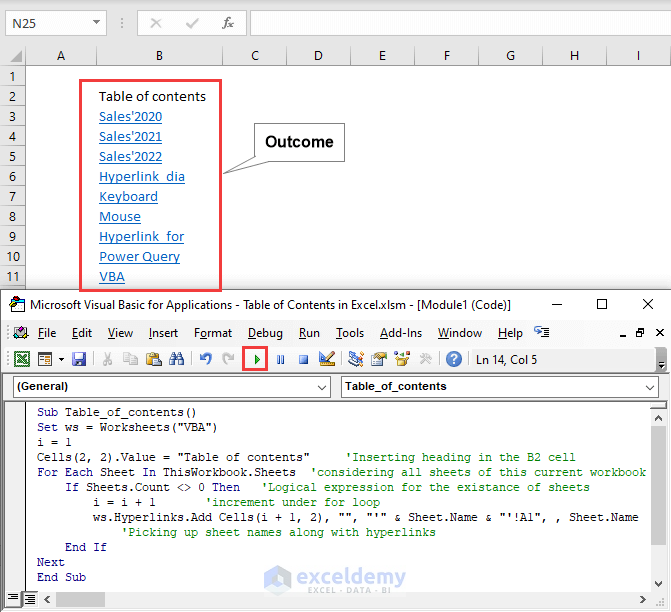
Code Breakdown
- We create a sub-procedure named Table_of_contents.
Sub Table_of_contents()

End Sub- Next, we set ws as VBA_event worksheet where the code runs. Also we insert a heading in the B2 cell.
Set ws = Worksheets("VBA")
Cells(2, 2).Value = "Table of contents"- Now, we use the For loop to consider all sheets of this current workbook. So, declaring the sheet as a worksheet object.
For Each Sheet In ThisWorkbook.Sheets
Next- We create a table of contents including hyperlinks based on a logical IF statement. If sheets are not 0 then we add worksheet names including their link in new cells using VBA Hyperlink properties.
i = 1
If Sheets.Count <> 0 Then
i = i + 1
ws.Hyperlinks.Add Cells(i + 1, 2), "", "'" & Sheet.Name & "'!A1", , Sheet.Name
End If
How to Create Dynamic Table of Content in Excel
If you add or remove worksheets, the previous methods can’t update the table of contents automatically. However, by applying the Named Range and VBA Macro tool, we can add or remove worksheets into the table of contents automatically. Keep in mind, that these approaches add hidden worksheets too.
1. Using Named Range with Formula
By defining the name of worksheets using the Define Name command, we will use a combined formula through which we can create the table of contents for each worksheet. This method shows the hidden worksheet after unhidden worksheets.
The functions we are going to use are REPT, NOW, SHEETS, ROW, SUBSTITUTE, HYPERLINK, TRIM, RIGHT, and CHAR functions.
Now check out the steps:
- First, select as follows: Formula >> Defined Names >> Define Name.
- Thus Edit Name dialog box appears. Put Sheet_Name as the name and write the following formula in the Refers to section >> hit OK command.
=GET.WORKBOOK(1)&REPT(NOW(),)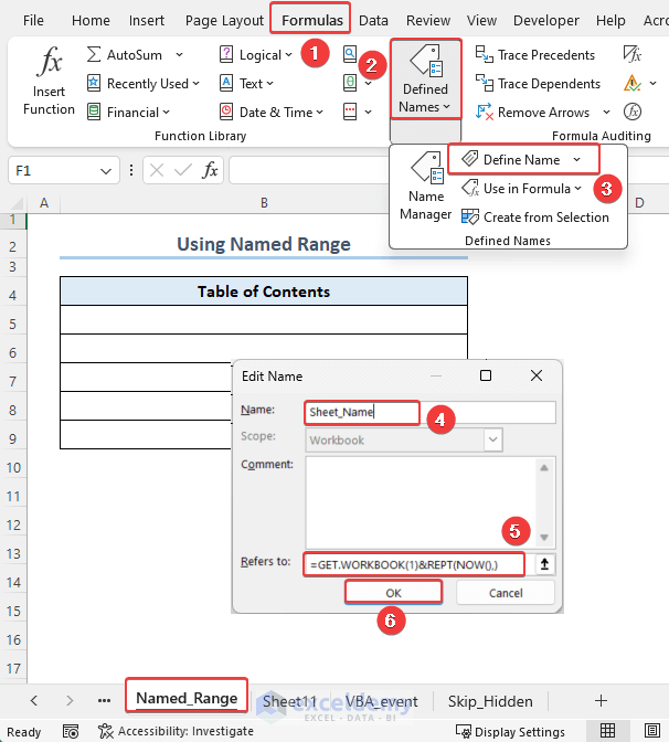
- Insert the following formula in the B5 cell.
=IF(ROW(A1)>SHEETS(),REPT(NOW(),),SUBSTITUTE(HYPERLINK("#'"&TRIM(RIGHT(SUBSTITUTE(SUBSTITUTE(INDEX(Sheet_Name,ROW(A1))," ",CHAR(255)),"]",REPT(" ",32)),32))&"'!A1",TRIM(RIGHT(SUBSTITUTE(SUBSTITUTE(INDEX(Sheet_Name,ROW(A1))," ",CHAR(255)),"]",REPT(" ",32)),32))),CHAR(255)," "))- Further, using the Fill Handle tool, we will be able to get the table of contents for worksheets.
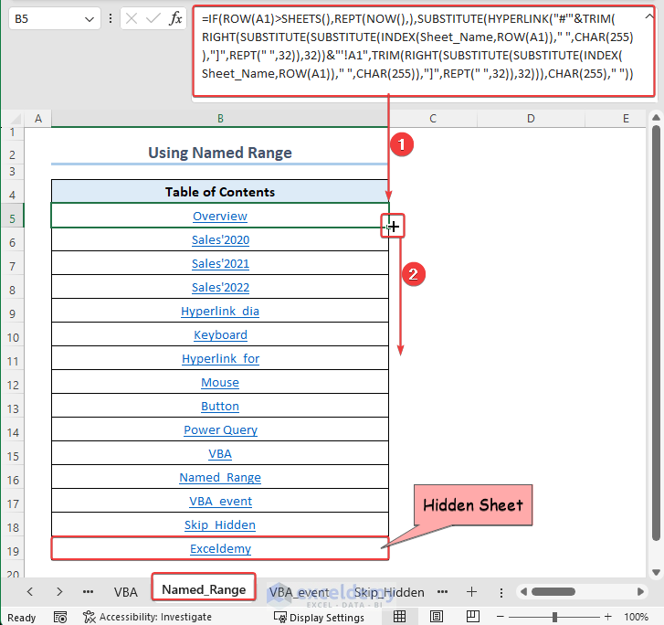
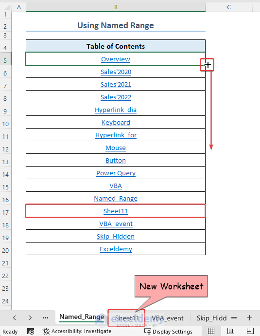
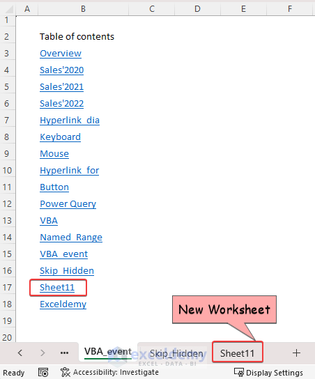
Therefore, after adding Sheet11, we obtain the sheet in the table of contents as well.
2. Applying VBA Code
Applying the VBA Activate event, we can create a dynamic table of contents. It can add or remove worksheets directly table of contents based on worksheet availability. Like the previous method, this approach also shows the hidden worksheet after unhidden worksheets. However, you don't need to press the Run command to execute the VBA code since the table of contents updates automatically.
- In the beginning, write the following VBA code in the worksheet module and save the file.
Option Explicit

Private Sub Worksheet_Activate()
Call Table_of_contents
End Sub

Sub Table_of_contents()
Dim ws  As Worksheet
Dim i As Integer
Dim sheet As Worksheet
Set ws = Worksheets("VBA_event")
ws.Cells.Clear
i = 1
Cells(2, 2).Value = "Table of contents"
For Each sheet In ThisWorkbook.Sheets
    If Sheets.Count <> 0 Then
        i = i + 1
        ws.Hyperlinks.Add Cells(i + 1, 2), "", "'" & sheet.Name & "'!A1", , sheet.Name
    End If
Next
End Sub
Click for a detailed view
Code Breakdown
- We create a sub-procedure named Table_of_contents.
Sub Table_of_contents()

End Sub- Next, we set ws as the VBA_event worksheet where the code runs. Also, we insert a heading in the B2 cell.
Dim ws  As Worksheet
Set ws = Worksheets("VBA_event")
Cells(2, 2).Value = "Table of contents"- Now, we use the For loop to consider all sheets of this current workbook. So, declaring the sheet as a worksheet object.
Dim sheet As Worksheet
For Each sheet In ThisWorkbook.Sheets
Next- We create a table of contents including hyperlinks based on a logical IF statement. If sheets are not 0 then we add worksheet names including their link in new cells using VBA Hyperlink properties.
Dim i As Integer
i = 1
If Sheets.Count <> 0 Then
i = i + 1
ws.Hyperlinks.Add Cells(i + 1, 2), "", "'" & sheet.Name & "'!A1", , sheet.Name
End If- The code may run several times. So, we clear the cells each time.
ws.Cells.Clear- We call the Table_of_contents sub procedure using the Call property enabling the Activate event in a private sub procedure.
Private Sub Worksheet_Activate()
Call Table_of_contents
End Sub- Thus, we obtain the table of contents including hidden Exceldemy worksheet.

- If we add a new worksheet it automatically shows up in the table of contents. But the hidden worksheet takes place after the unhidden worksheets.
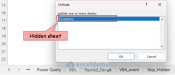
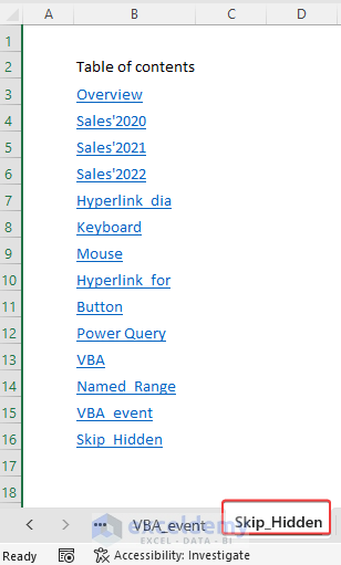
How to Skip Hidden Sheets from Table of Contents in Excel
Here, we have a hidden worksheet named Exceldemy. We will make a table of contents skipping the Exceldemy worksheet by using the sheet.Visible property. You need to click the Run command every time to execute the VBA code.
- Write the following VBA code in the Module and hit the Run command.
Sub Skip_Hidden_Worksheets()
Dim ws As Worksheet
Dim i As Integer
Dim sheet As Worksheet
Set ws = Worksheets("Skip_Hidden")
ws.Cells.Clear
i = 1
Cells(2, 2).Value = "Table of contents"
For Each sheet In ThisWorkbook.Sheets
    If sheet.Visible = xlSheetVisible Then
        i = i + 1
        ws.Hyperlinks.Add Cells(i + 1, 2), "", "'" & sheet.Name & "'!A1", , sheet.Name
    End If
Next
End Sub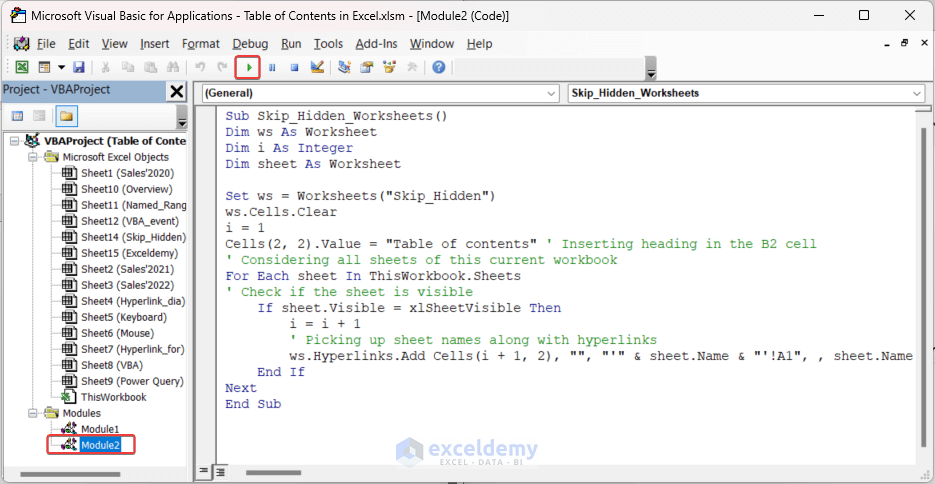
Code Breakdown
If you observe closely, you will notice that our code is almost similar. But there is a little change. The Sheet.Visible property helps to skip the hidden worksheet. The property judges based on the worksheets’ visibility.
If sheet.Visible = xlSheetVisible Then
i = i + 1
ws.Hyperlinks.Add Cells(i + 1, 2), "", "'" & sheet.Name & "'!A1", , sheet.Name
End If
- Subsequently, we get the output avoiding the hidden Exceldemy sheet.
Read More: Make Table of Contents Using VBA
Things to Remember
- To open the Hyperlink dialog box, you can press Ctrl + K from the keyboard.
- The HYPERLINK function to add links to the table of contents.
- The Mouse Cursor method inserts a hyperlink to an existing text.
- Power Query and Excel VBA Macro tools develop a table of contents automatically.
- Named Range and VBA Activate event helps to update the table of contents automatically.
- Visible property in VBA is used to show hidden worksheets.
Frequently Asked Questions
1. Can I create a table of contents if I have only one sheet?
Answer: Yes, you can create a table of contents containing one worksheet only using the HYPERLINK function, Inert hyperlink dialog box, and so on.
2. Can the table of contents update itself after adding a new worksheet?
Answer: Yes, you can automate a table of contents in Excel using the Worksheet Activate event or Named Range tool. Thus the table of contents will update automatically after adding or removing a new worksheet every time.
3. How do I add two tables of contents in Excel?
Answer: Excel doesn't have a built-in feature to add two or multiple tables of contents at the same time. However, you can create multiple tables of contents in multiple columns using VBA Macro automatically. Further, the use of the HYPERLINK function can be useful to add manually.
4. Doesn't Microsoft Excel do the same without any add-ins?
Answer: No, Excel doesn't have any built-in way to generate a table of contents. The job is done with a VBA code, Insert Hyperlink dialog box, or HYPERLINK function to create a table of contents.
5. Is there a limit to the number of sheets to create a table of contents?
Answer: No there is no limit to the number of sheets to create a table of contents. However, application of VBA Macro tool is suitable for a workbook containing numerous worksheets.
Download Practice Workbook
Conclusion
Throughout the article, we provided a short and complete guideline with where the use of the Insert Hyperlink dialog box, keyboard shortcut, Mouse Cursor, and HYPERLINK function shows the approaches to construct a table of contents manually in Excel. On the other hand, using the Power Query and VBA Macro tool you can prepare a table of contents automatically. In addition, VBA Macro, as well as Named Range, are useful tools for developing a dynamic table of contents. Don’t forget to leave your thoughts in the comment section. Hope to catch you soon with any other new content.
Table of Contents in Excel: Knowledge Hub
- Create Table of Contents Without VBA
- Create Table of Contents in Excel with Page Numbers
- Create Table of Contents for Tabs
<< Go Back To Hyperlink in Excel | Linking in Excel | Learn Excel

