Gridlines in Excel Chart

Get FREE Advanced Excel Exercises with Solutions!

This article focuses on gridlines in Excel. These are important features that play a significant role in enhancing the readability of chart and graphs. The horizontal and vertical lines make a grid-like pattern which helps to align and compare data and identify trends.

In this article, we will explore gridlines in Excel chart. We will start this article by explaining how to chart gridlines in two easy ways- using the Chart Design tab and the Chart Elements button.

Then we will move on to discuss how to format chart gridlines for both solid (major axis) lines and gradient (for minor axis) lines. Finally, we will wrap up by describing how to remove gridlines from Excel chart.

Download Practice Workbook

Download this practice workbook while reading this article.

Gridlines_in_Excel.xlsx

Table of Contents Expand

What Are Gridlines in Excel Chart?

Gridlines are horizontal and vertical lines drawn from both axes that pass through each other, creating a grid-like pattern. They are drawn to make it easier to read and interpret data points represented in a chart.

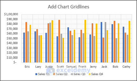
How to Add Chart Gridlines

In this example, we will explain how to add chart gridlines in Excel in two easy ways- from ribbons and, for later versions of Excel, the Chart Elements button. It will only be available on the ribbon once you have selected the chart on your spreadsheet.

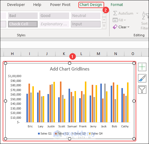
1. Add Gridlines From Ribbon

You can add chart gridlines from the Chart Design tab of the Excel Ribbon.

First, select the chart and then click on the Chart Design tab.

Add Major Gridlines:

To add Major Gridlines, go to Add Chart Element >> Gridlines.
Then select Primary Major Horizontal and Primary Major Vertical to add major gridlines.

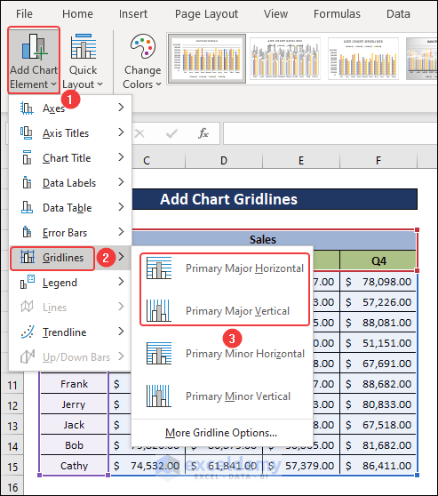
As a result, major gridlines will be added.

Add Minor Gridlines:

Similarly, if you want to add Minor Gridlines, select Primary Minor Horizontal and Primary Minor Vertical.

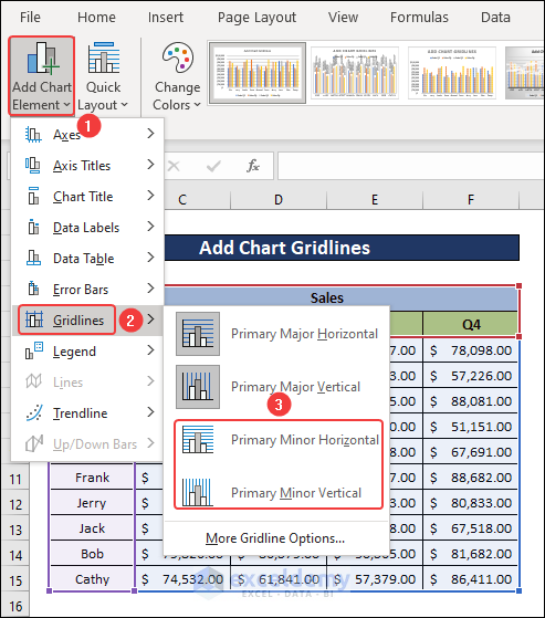
Consequently, minor gridlines will be added.

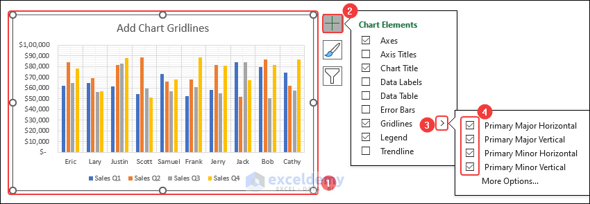
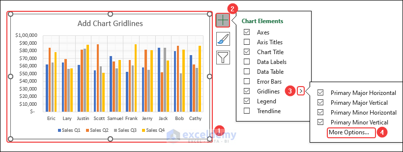
2. Using Chart Elements Button

Gridlines can also be added using the Chart Elements button. These are the buttons that appear on the right side of the chart once you have selected it in the spreadsheet.

The steps to do so are discussed below.

First, click on the chart and select the Chart Elements button.
Then click on the arrow beside Gridlines.
After that, Check the gridline options you want to add.

Consequently, gridlines will be added.

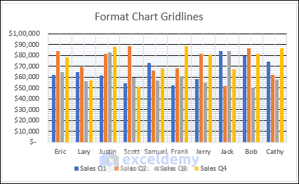
How to Format Chart Gridlines

There are several options that can help improve the appearance of the chart. One of them is chart gridlines format options.

After clicking on the Chart Elements button, go to Gridlines >> More Options to open the Format Gridlines panel.

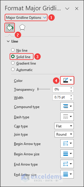
Formatting Solid Gridlines in Excel Chart

We are selecting Major Gridline Options from the dropdown for the Solid Line options’ demonstration.

Select Major Gridline Options from the dropdown.
Then choose the Fill & Line tab.
Select Solid Line and change the Color as per your need.

Formatting Gradient Gridlines in Excel Chart:
We will format minor gridlines as gradient lines.

Choose Minor Gridline Options from the dropdown.
Select the Gradient line and any of the Preset gradients.

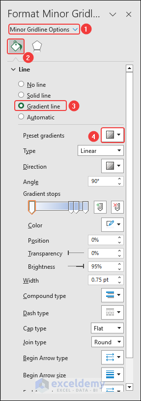
Finally, the output will look like the following image.

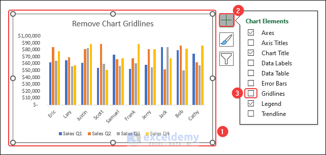
How to Remove Chart Gridlines

Removing chart gridlines is an easy task. First, select the chart and click on the Chart Elements button. Then uncheck the box of Gridlines.

Things to Remember

Choose a color for gridlines that does not clash with the data points or other visual elements.
You can enable and disable gridlines series by series basis.
While printing the charts, make sure to the gridlines are visible on your printing options.

Conclusion

Thanks for reading this article. I hope you found this article useful. In this article, we have explained how to add chart gridlines in Excel in two ways. We have also described how to format and remove gridlines. If you have any queries or recommendations regarding this article, feel free to let us know in the comment section below.

Frequently Asked Questions (FAQs)

1. Why can’t I see gridlines in Excel?

Go to the View tab and check the box of Gridlines to show gridlines. If the cell fill color is white instead of No Fill, it will appear that the gridlines are missing. Change the cell fill color to No Fill to solve this problem.

2. What Color are gridlines in Excel?

Excel gridlines are of light gray color by default. However, it is possible to change this color. Go to, File >> Excel Options >> Advanced >> Display Options for the Worksheets >> Select the Gridline Color.

3. What does gridlines print do in Excel?

Gridlines are modeled to print around only actual data in a worksheet. You can see the preview before printing a worksheet by going to the Layout tab. Then under Print, click Preview.