Split Column in Excel

Get FREE Advanced Excel Exercises with Solutions!

In this article, we are going to see how we can split columns in Excel using various methods. In Excel, we need to split columns on many occasions. Sometimes based on a delimiter or sometimes based on a fixed width. Below, we will show methods and discuss how we can split a single column to multiple columns using functions, features, power query, and VBA macro in Excel.

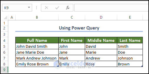
Below we are showing a sample of how we can split columns in Excel using Power Query.

Download Practice Workbook

Download this practice workbook below.

Split Column.xlsm

Table of Contents Expand

How to Use Excel Features to Split Columns in Excel

We will show various methods to split columns in Excel, among them are the Text to Columns feature, the Flash Fill feature, and multiple function usage. In order to avoid the compatibility issue, users are advised to use the Excel 365 edition.

1. Using Text to Columns Command

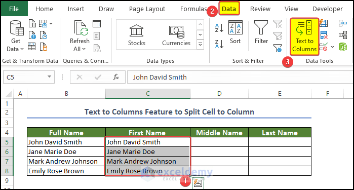
Users can use the Text to Column feature to Split the cell value into different columns. Firstly, the user must first copy the text content in the range of cells B5:B8. And paste them into the field of cell C8.

Then go to the Data tab > Text to Columns.

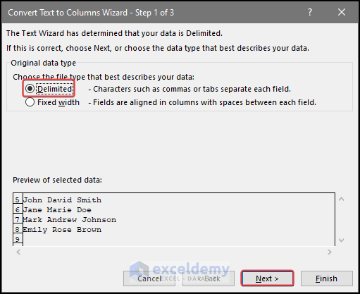
After that, there will be a window, and we need to select the Delimited in the Choose the file type that best describes your data:
Right after that, Click on the Next.

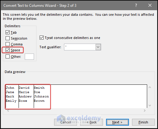
Then we need to check the box in the space box in the delimiter section.
Click on the Next options.

Then, in the window, we will select the General option in the Column data format.
Click on the Finish after this.

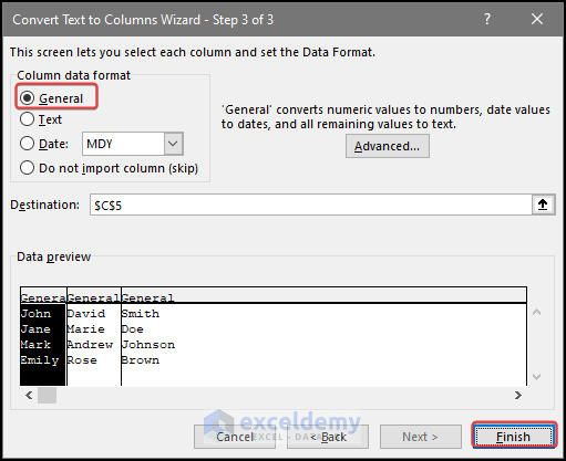
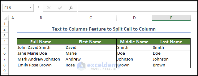
After this, we will see that the full name is now split into three separate columns.

2. Using Flash Fill Feature in Excel

In this method, we can use the Flash Fill Feature to split cell values into columns.

We now need to fill out the column cell values in the same format as you want them.
Meaning the way the user wants to separate the full name into separate columns.
For example, we have the full name John David Smith in cell B5.
We need to separate the names into First name, Middle name, and Last name.
So we place the name accordingly in cell C5:E5.

After that, we will hold on to the right mouse button on the corner of cell C5 in the worksheet. We will see that plus icon in the corner.

Then we need to drag that icon to cell C8.
After dragging the icon to cell C8, release the mouse button.
Then we can see that there is a context menu.
In the context menu, click on the Flash Fill option.

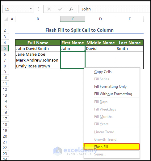
After this, we will see the output with the separated first part of the names.

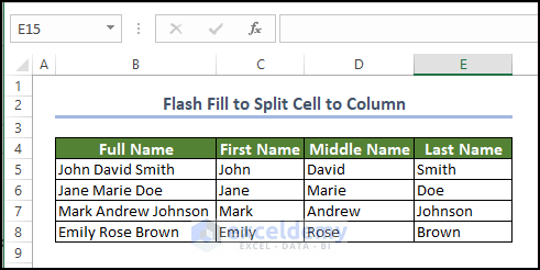
Repeat the same process for the rest of the columns.
The final output will be look something like the below.

How to Use Functions to Split Columns in Excel

We can use a wide variety of Functions to split columns in Excel. For example, we can use the LEFT, and the FIND function to split the columns in Excel.

1. Combining Multiple Functions to Split the First/Middle/Last Text of a Column

We can combine or use different variations of functions and formulas in Excel to split various parts of the text available.

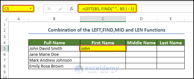
For example, if we want to extract the first part of the full name, we can enter the following formula in cell C5.

=LEFT(B5, FIND(" ", B5 ) - 1)

Press Enter after this.

Then drag the fill handle to cell C8.
Then, to extract or split only the middle part of the name from the full name, enter the following formula in cell C8.

=MID(B5, FIND(" ", B5) + 1, FIND(" ", B5, FIND(" ", B5) + 1) - FIND(" ", B5) - 1)

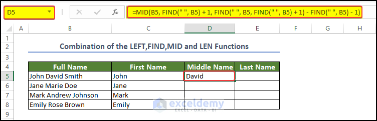
Then drag the fill handle to cell D8.
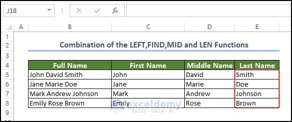
Up next, to get the last part of the name, enter the following,

=RIGHT(B5,LEN(B5)-FIND(" ",B5,FIND(" ",B5)+ 1))

Then drag the fill handle to cell E8.
After this, we will notice that the range of cell C5:E8 is now filled with the split name from the Full name mentioned in the range of cell B5:B8

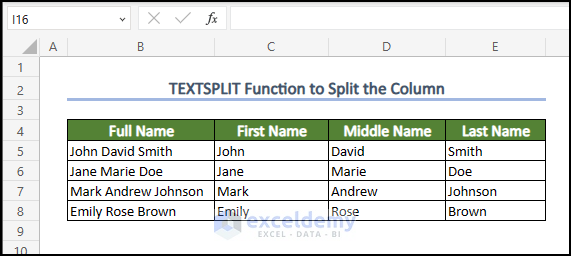
2. Using TEXTSPLIT Function

We will use a function named TEXTSPLIT to split the names according to the delimiter.

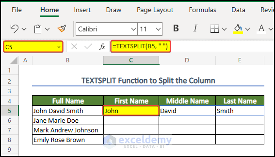
We have the full name in the range of cells B5:B8, we need to split the names into different parts.
For this, enter the following formula in cell C5,

=TEXTSPLIT(B5, " ")

Immediately after entering the formula and pressing the enter button on the keyboard, we will see that the split name parts are present in the range of cells C6:E5.

Then drag the fill handle to cell C8.
After that, the range of cells C5:E8 will be filled with the first and last names of the Full name presented in the range of cell B5:B8.

Note:

Unfortunately, this function is only available in Excel 365

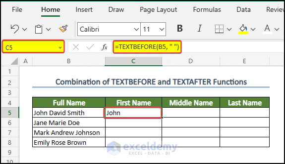
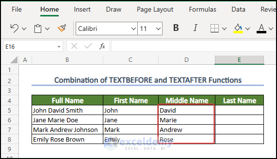
3. Combining TEXTBEFORE and TEXTAFTER Functions

We can use the combinations of TEXTBEFORE and TEXTAFTER functions to split the names of people stated in the range of cells B5:B8.

For this, enter the following formula in cell C5,

=TEXTBEFORE(B5, " ")

Press Enter after this.
We will see the First name in cell C5.

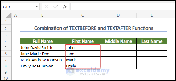
Then we can drag the fill handle to cell C8.
We will see that the range of cell C5:C8 is now filled with the first name of the person.

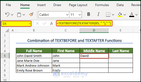
To split out the middle part of the name, users can enter the following formula in cell D5,

=TEXTBEFORE(TEXTAFTER(B5, " ")," ")

Press Enter after this.
After pressing Enter, you will see the middle part of the name split out in cell D5.

Then drag the fill handle to cell D8.
We will see that the range of cells D5:D8 is now filled with the middle part of the name mentioned in the range of cells B5:B8.

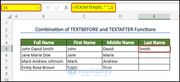
We will enter the following formula in cell E5:

=TEXTAFTER(B5, " ",2)

Press Enter after this.
After pressing Enter, we will notice the last part of the name present in cell E5.

Drag the Fill Handle to cell E8.
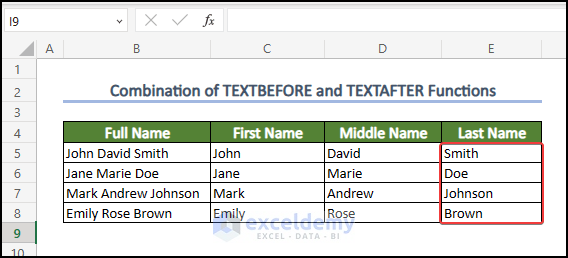
After then, we will notice that the range of cells E5:E8 is now filled with the last part of the name mentioned in the range of cells B5:B8.

Note:

Unfortunately, this function is only available in Excel 365 edition.

How to Use Power Query to Split Columns in Excel

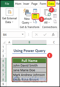
In the below method, we are going to use Power Query to split columns in the Excel worksheet.

First, select the range of cells B4:B8 and then go to the Data tab > Get and Transform Data group > From Table/Range.

Then we will see a Power Query window appear where we can see that the table that we chose previously is now present.
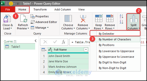
Then we go to the Home tab and click on the Split Column
After clicking on the Split Column option, the user can see a drop-down option.
In the drop-down option, select the Delimiter option.

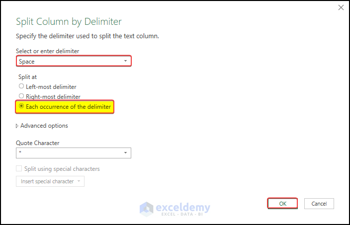
After selecting the Delimiter option, we can see that there is a window named the Split Column by Delimiter.
In that window, choose the Space as Delimiter option from the Select or Enter Delimiter option.

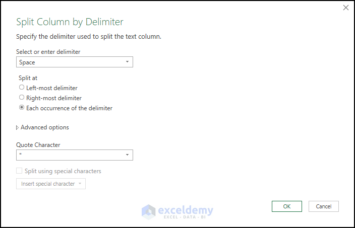
After then, select Each occurrence of the delimiter on the Split at
The rest of the options should stay unchanged.
Click OK after this.

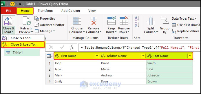
After then, we will see the names are now split into three different parts in the power query editor.

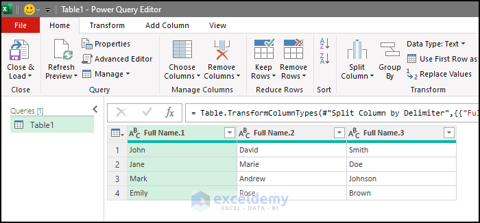
Now we need to load this table back into the worksheet. But first, we need to update the table header names.
Change the table header as shown in the image below and then go to the Home tab > Close & Load to > Close & Load To…

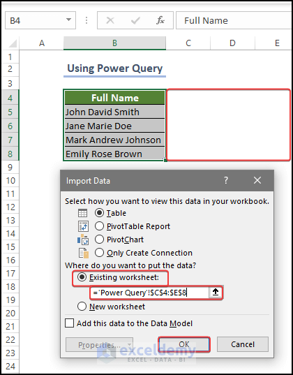
Then we will switch to the worksheet, and on the worksheet, we are going to see a window.
In the window, we will select Table in the Select how you want to view this data in the workbook
Then select Existing worksheet in the Where do you want to put your data.
Then set the range of cells to C4:E8.
Click OK after this.

After loading the sheet into the worksheet, we can see that the table is now present in the worksheet. Where the name is now split into three separate parts.

How to Use VBA Macro to Split Column in Excel

We can use a simple VBA macro to split column values into different columns.

We have the full names of the people in the range of cells B5:B8.

For this, we first need to initiate the code editor following the helper article given here.
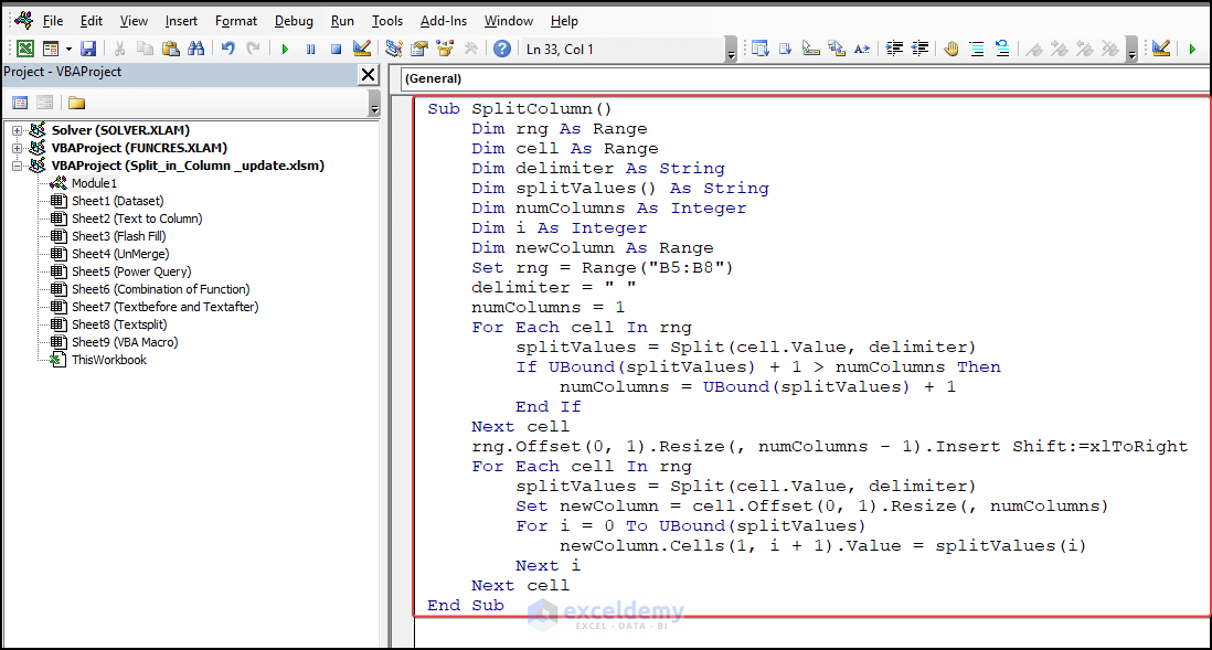
In the code editor, enter the following code:

Sub SplitColumn()
    Dim rng As Range
    Dim cell As Range
    Dim delimiter As String
    Dim splitValues() As String
    Dim numColumns As Integer
    Dim i As Integer
    Dim newColumn As Range
    Set rng = Range("B5:B8")
    delimiter = " "
    numColumns = 1
    For Each cell In rng
        splitValues = Split(cell.Value, delimiter)
        If UBound(splitValues) + 1 > numColumns Then
            numColumns = UBound(splitValues) + 1
        End If
    Next cell
    rng.Offset(0, 1).Resize(, numColumns - 1).Insert Shift:=xlToRight
    For Each cell In rng
        splitValues = Split(cell.Value, delimiter)
        Set newColumn = cell.Offset(0, 1).Resize(, numColumns)
        For i = 0 To UBound(splitValues)
            newColumn.Cells(1, i + 1).Value = splitValues(i)
        Next i
    Next cell
End Sub

After entering the code, press Enter.

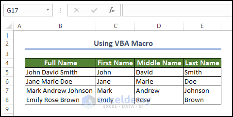
After pressing Enter, the user will notice that the full name in the range of cell B5:B8 is already split into three separate columns.

VBA Code Breakdown

Sub SplitColumn():

This line starts the declaration of a subroutine called “SplitColumn.”

Dim rng As Range:

Declares a variable named “rng” of type Range. This variable will be used to store a range of cells.

Dim cell As Range:

Declares a variable named “cell” of type Range. This variable will be used to iterate through each cell in the range.

Dim delimiter As String:

Declares a variable named “delimiter” of type String. This variable will store the delimiter used to split the cell values.

Dim splitValues() As String:

Declares a dynamic array named “splitValues” that will store the values obtained after splitting a cell’s value.

Dim numColumns As Integer:

Declares a variable named “numColumns” of type Integer. This variable will store the number of columns needed to accommodate the split values.

Dim i As Integer:

Declares a variable named “i” of type Integer. This variable will be used as a loop counter.

Dim newColumn As Range:

Declares a variable named “newColumn” of type Range. This variable will store the range of cells where the split values will be placed.

Set rng = Range(“B5:B8”):

Sets the “rng” variable to represent the range of cells B5 to B8.

delimiter = ” “:

Sets the “delimiter” variable to a space character, indicating that the cell values will be split based on spaces.

numColumns = 1:

Sets the initial value of “numColumns” to 1.

For Each cell In rng:

Starts a loop that iterates through each cell in the range represented by “rng.”

splitValues = Split(cell.Value, delimiter):

Splits the value of the current cell using the specified delimiter and stores the resulting values in the “splitValues” array.

If UBound(splitValues) + 1 > numColumns Then:

Checks if the number of split values is greater than the current value of “numColumns.”

numColumns = UBound(splitValues) + 1:

If the number of split values is greater, update the value of “numColumns” to the new maximum.

Next cell:

Ends the loop and proceeds to the next cell in the range.

rng.Offset(0, 1).Resize(, numColumns – 1).Insert Shift:=xlToRight:

Inserts a new range of cells to the right of the original range, with the number of columns equal to “numColumns – 1.”

For Each cell In rng:

Starts a new loop to iterate through each cell in the original range.

splitValues = Split(cell.Value, delimiter):

Splits the value of the current cell using the specified delimiter and stores the resulting values in the “splitValues” array.

Set newColumn = cell.Offset(0, 1).Resize(, numColumns):

Sets the “newColumn” variable to represent the range of cells starting from the cell one column to the right of the current cell, with a width equal to “numColumns.”

For i = 0 To UBound(splitValues):

Starts a loop that iterates through each element in the “splitValues” array.

newColumn.Cells(1, i + 1).Value = splitValues(i):

Assigns the i-th value from the “splitValues” array to the corresponding cell in the “newColumn” range.

Next i:

Ends the loop and proceeds to the next element in the “splitValues” array.

Next cell:

Ends the loop and proceeds to the next cell in the range.

End Sub:

Marks the end of the subroutine “SplitColumn.”

Things to Remember

Choose the appropriate delimiter: Determine the delimiter character that separates the values

Consider data validation: If your data has specific formatting or validation rules applied, such as data types, formulas, or conditional formatting, be cautious when splitting the column. Ensure that the resulting split columns preserve the data validation and formatting rules. You may need to reapply any necessary validation or formatting to the new columns.

Insert new columns: Decide where you want the split values to be placed. It’s generally a good practice to insert new columns adjacent to the original column, rather than overwriting or replacing the existing data. This allows you to preserve the original data and easily revert back if needed.

Check data types: After splitting the column, verify that the data types in the split columns are correct. Sometimes, Excel may automatically format the split values as dates or numbers, even if they were originally text. Adjust the data types as needed to maintain the desired formatting.

Frequently Asked Questions

Q1. Can you split a single column in Excel?

To split a cell into two smaller cells within a single column in Excel, you’ll need to follow a workaround since Excel doesn’t provide a direct feature for this. First, create a new column next to the column containing the cell you want to split. Then, you can proceed to split the cell by either copying its contents into the new adjacent cell or dividing the content into multiple adjacent cells. By utilizing this method, you can achieve the desired split while working within a single column.

Q2. What is the shortcut to split columns in Excel?

In Excel, there is a shortcut to split columns called “Text to Columns.” The shortcut key combination to access this feature is:

Alt + A + E

By pressing these keys together, you can quickly open the “Convert Text to Columns” wizard, which allows you to split the contents of a column based on a specified delimiter. Moreover, this shortcut is applicable to most versions of Excel.

Q3. How do I split a column by position in Excel?

Open Excel and open the workbook that contains the column you want to split.

Select the column that you want to split by clicking on the column header.
After this, Go to the “Data” tab in the Excel ribbon at the top.
In the “Data Tools” group, click on the “Text to Columns” button. This will open the “Convert Text to Columns Wizard” window.
In the wizard, you’ll see two options for splitting the column: “Delimited” and “Fixed width.” Since you want to split by position, choose the “Fixed width” option and click “Next.”
Then you can see that a vertical line appears and using that line, you can manually set the width of the character spacing.