Excel Unique Values

In this article, we have demonstrated all the necessary information that is related to Excel unique values. We will use functions and pivot table to demonstrate how to find unique values. Furthermore, learn all the ways to use the UNIQUE function to find unique values in Excel.

Unique values are crucial in all professions. Starting from data management and analysis to the decision-making process, unique values offer deeper insights, important information, trends, patterns, and diversity. Therefore, in Excel, professionals often require different kinds of analysis or financial modeling depending on various purposes. We hope you can take away all the information and be able to use it in your work for better and more efficient outcomes.

How to Find Unique Values in Excel: 3 Suitable Ways

In Excel, there are different ways to find unique values, depending on the purpose and the dataset. You can use a toolbox, pivot table, Excel function, or other Excel features as per your preference.

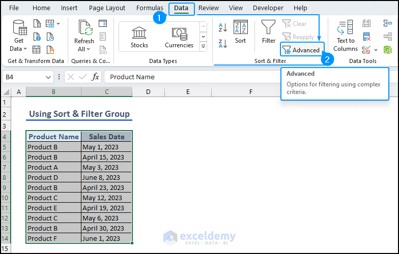
1. Using Sort & Filter Group

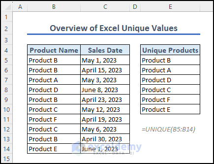
Assume that we have the following dataset that contains the names of the products and their sales date. We will use this dataset to find unique values in Excel.

Start by selecting the range of data and navigating to the Data tab. In the Sort & Filter group, choose the Advanced option. (Click on the image for clear visualization)

Within the Advanced Filter window, you have two choices. You can either filter the data within the existing range or copy it to a different location. In this case, we will filter within the existing range.

Make sure to select the “Unique records only” checkbox to filter for unique values. Finally, click the OK button to apply the filter.

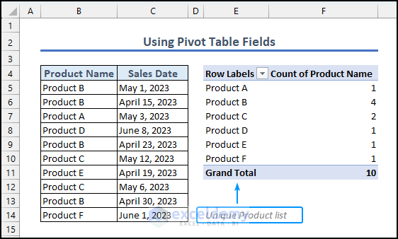
2. Using Pivot Table Fields

Another method to find and count unique values in Excel is by using a pivot table. We will use the previous dataset to demonstrate the process.

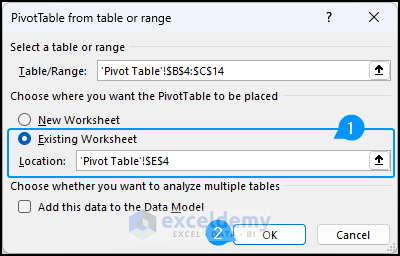
Select the range of data and then go to the Insert tab in Excel. From the drop-down menu of the PivotTable option, select From Table/Range.

A new window will appear. Choose the location for the pivot table, such as the existing worksheet where the location is cell G5. Finally, click OK to create the pivot table.

On the left side of the window, you will see the PivotTable Fields section. Select the Product Name and drag it to both the Rows and Values field boxes.

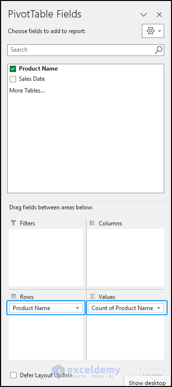
The pivot table will generate the output, showing the total count of unique products and the number of units sold for each product.

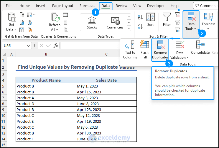
3. Find Unique Values by Removing Duplicate Values

We can find unique values in Excel by removing duplicate values. We can use the built-in “Remove Duplicates” feature. Once again using the same dataset, we will demonstrate the process.

Select the data range and go to the Data tab in Excel. In the Data Tool group, click on the Remove Duplicates button.

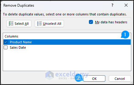
From the Remove Duplicate dialogue box, select the column that has duplicate values, such as the Product Name column. Make sure the “My data has headers” option is checked if your range includes headers. Click OK to continue.

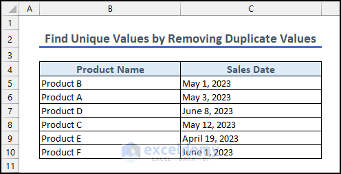
It will show the following notification after removing all the duplicates.

We will have the following output, where we will find all the unique products.

How to Use UNIQUE Function to Find Unique Values for Multiple Criteria: 12 Useful Methods

In the updated versions of Excel, such as Excel 365, the UNIQUE function is available to find unique values in a dataset. Besides, The UNIQUE function offers various uses and can be applied in multiple ways. Check out the following section to learn all the ways to use the UNIQUE function in Excel.

Method 1: Find Unique Values

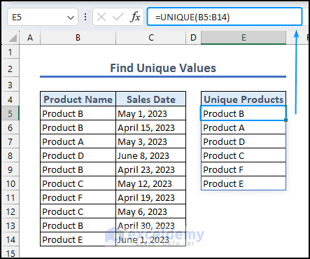
We will use the following dataset to find the unique products by using the UNIQUE function.

First, select cell E5 under the Unique Products column and type the following formula.

Then press ENTER and you will see that it will return a list of all the unique products available in the dataset.

Read More: How to Get Unique Values in Excel

Method 2: Combining SORT & UNIQUE Functions

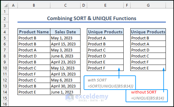
We can sort the output result of the UNIQUE function with the help of the SORT function. Once again, we will use the same dataset to demonstrate the process.

First, select cell E5, and then we will use the following formula.

Finally, pressing ENTER will provide the following output.

As observed, the SORT function takes the values returned by the UNIQUE function and arranges them in sorted order, resulting in the updated output.

Method 3: Using UNIQUE Function to Concatenate Unique Values

We will use the following dataset to show how to use the UNIQUE function to merge or concatenate texts in Excel.

First, we will select cell E5 and then apply the following formula.

After pressing ENTER, the formula will generate the output as shown in the image. The previously separate columns for first name and last name are now combined to form the full name.

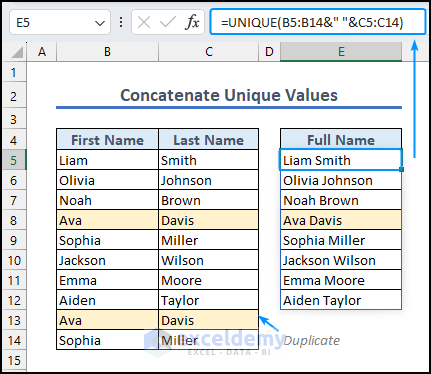
If there are repetitions in the names, the formula will ignore the names that appear more than once in the data, for example, Ava Davis. It will only consider unique names when combining them into the full name.

Method 4: Find Unique Values by Comparing Two Columns

We can also use the UNIQUE function to find unique values in two or more columns. Check out the following example.

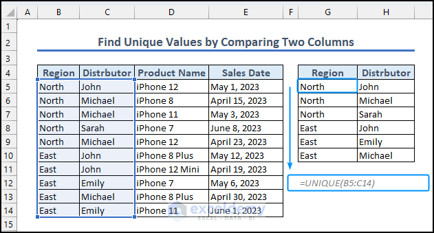
Assume that in the following dataset, there are two columns containing the names of the regions and the distributors‘ names. We are going to find the regions and unique distributors in each region.

Once again, select cell G5 and use the following formula.

It will return the following output. You will see that it lists the regions and, beside them, the unique distributor names.

Read More: Create List of Unique Values from Multiple Sheets

Method 5: Find Unique Values Along Rows

Consider that we have the following dataset that contains the hourly sales time and the device name that was sold within the observation week. We are going to use this dataset to demonstrate how to find unique values in rows.

First, select the cell in C18 and use the following formula.

The second argument in the UNIQUE function is optional. If the by_col parameter is set to TRUE it will consider each column to be separated and return unique values for each column.

Thus, it returned the unique products that were sold on May 1, 2023, which are the iPhone 8 and iPhone 12. These two products were the only ones sold throughout the entire day of work.

Method 6: Find Unique Values That Appeared Exactly Once

Assume that we have the following dataset, and we want to find the devices that were sold only once within this sample dataset.

Start by selecting cell E5, and we will use the following formula.

Here, the third argument, exactly_once in the UNIQUE function is also optional. If this is set to TRUE it will return the unique values that appeared in the dataset just once.

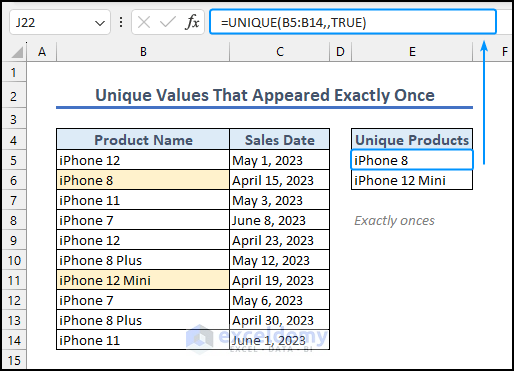
By checking the output, it becomes evident that there are only two specific phone models, namely the iPhone 8 and the iPhone 12 Mini, that were sold only once within the observed time period.

Read More: VBA to Get Unique Values from Column into Array

Method 7: Combining UNIQUE, FILTER, and COUNTIF Functions to Find Distinct Values with Multiple Entries

We can also find the values that occur more than once in a dataset. Using the same data, we will demonstrate the process.

First, select cell E5, and then we will use the following formula.

Finally, pressing ENTER will provide the following output.

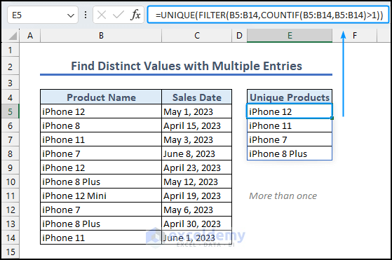
The formula finds and returns a list of unique values from the range B5:B14 that appear more than once in the range.

Method 8: Find Unique Values for Single Criteria

We can also find unique values based on different criteria. For example, assume that we use the following dataset to find the products in a specific category, such as Electronics.

Once again, we will select cell H5 and use the following formula.

Finality, press ENTER to get the result.

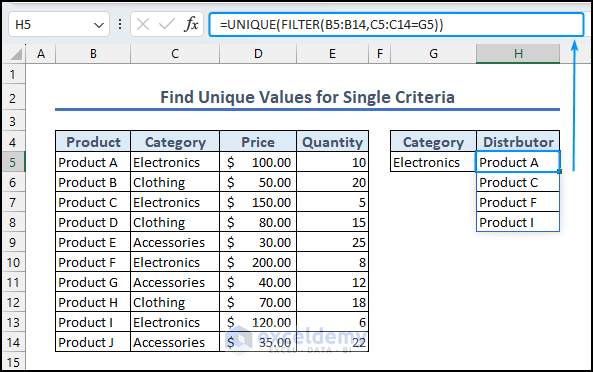
Here, the FILTER function filters the data range based on the criteria of whether it is equal to G5 or not, and in the end, the UNIQUE function returns the unique values, eliminating any duplicates.

Read More: Copy Unique Values to Another Worksheet in Excel

Method 9: Extract Unique Values with Multiple Criteria

We can also find unique values based on multiple criteria. We will use the following dataset to find the electronics products that have a price above $140 and a quantity less than 8.

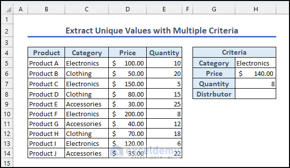
Begin by selecting cell H5 and using the following formula.

Finality, press ENTER to get the result.

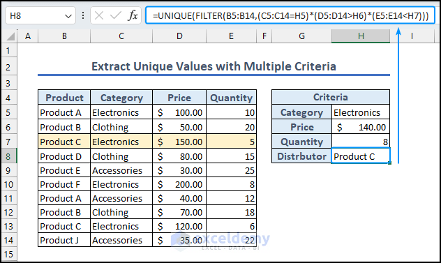
Multiple criteria are used within the FILTER function for filtering the data, and the UNIQUE function then returns the unique values from multiple criteria.

As a result, we have one product (Product C) that satisfies both criteria.

Method 10: Extract Unique Values with OR Criteria

We can also find unique values based on multiple OR criteria. For example, we are going to find unique products that are from the electronics and accessories category.

Once again, select cell H5 and use the following formula.

Finally, press ENTER to find the output.

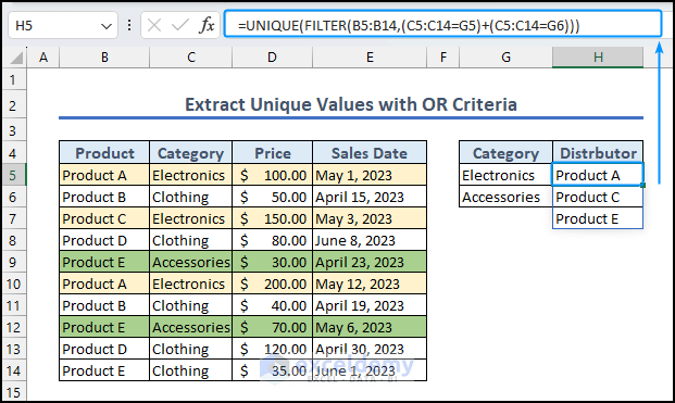
Thus, we find three products from two different categories that match the OR criteria.

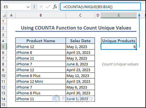
Method 11: Using COUNTA Function to Count Unique Values

If you want to count the number of unique values in the dataset, you can use the following formula.

For example, we used this dataset to count the total number of unique products. In cell E5, we used the following formula.

With the help of the COUNTA function, it returned the total number of unique values found in the dataset, which is 6.

Read More: Extract Unique Values Based on Criteria

Method 12: Find Unique Values in Excel by Ignoring Blank Cells

If your Excel dataset has blank cells, empty spaces, or zero values, you can use the following formula to avoid such information.

In cell D17, we used the following formula to avoid blank spaces and empty cells.

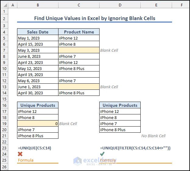
As a result, the formula returns an output that does not have any blank space or a zero value.

How to Handle Error Values While Looking for Unique Values

To handle situations where there are no unique values in a dataset and prevent error values, you can use the IFERROR function. This allows for smoother data analysis and prevents errors by providing a clear output.

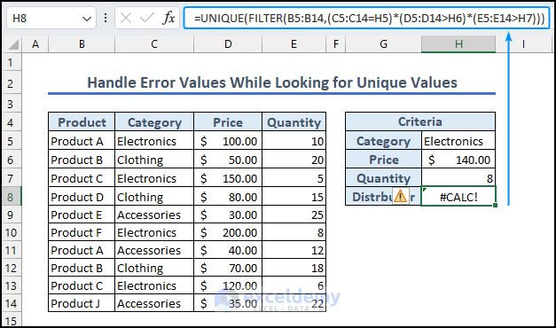
In our attempt to identify unique electronic products priced above $140 and with a quantity greater than 8, it was found that there are no products meeting these criteria. Therefore, instead of displaying an error message (#CALC!), the formula returns the message “No Unique Values“.

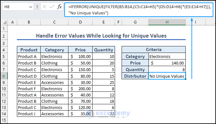
Things to Remember

• Distinct values refer to the total unique values available in a dataset. While unique values of a dataset refer to the values that appear only once in the dataset.
• While using the UNIQUE function, the results update automatically when the source data changes. Data change must be made within the cell reference.
• If your dataset contains blank cells, empty strings, or zero values, the UNIQUE function will include them in the output.

Download Practice Workbook

Conclusion

In conclusion, this article aimed to provide a clear understanding of the concept of unique values in Excel. Understanding the significance of Excel unique values is essential for effective data analysis, reporting, and decision-making processes.

Whether you need to extract distinct values, remove duplicates, or filter data based on uniqueness, Excel offers various tools and functions to accomplish these tasks.

If you like this article, check out Exceldemy for more relevant content.

Frequently Asked Questions

Q1. How can I find unique values in Excel without removing duplicates?
One way to find unique values without removing duplicates is by using the Advanced Filter feature, which allows you to copy unique values to another location while keeping the original dataset intact.

Q2. Which Excel versions support the UNIQUE function?
The UNIQUE function is available in Excel 365 and later versions. It is not available in earlier versions of Excel, such as Excel 2016, Excel 2013, Excel 2010, or Excel 2007.
If you have an older version of Excel, you may need to use alternative methods like the “Remove Duplicates” feature or formulas to find unique values.

Q3. How do I create a unique value table in Excel?
First, open your Excel worksheet and select the range of data that you want to extract unique values from. Go to the Data tab > Data Tools group, > click the Remove Duplicates button.

A dialog box will appear showing a preview of the selected range with checkboxes next to each column. Click the “OK” button. Excel will remove any duplicate values from the selected range.

Now, copy the remaining unique values and paste them into a new location in your worksheet to create the unique value table

Q4. How do I use unique filters in Excel?
Excel does not have a built-in unique filter feature. However, you can use the advanced filter option.
First, select the dataset, then go to the Data tab > from the Sort & Filter group > select Advanced > from the new dialogue box, and select Unique records only.

Excel Unique Values: Knowledge Hub

<< Go Back to Learn Excel