Filter in Excel means displaying only the data that meets certain criteria and hiding the rest of the data temporarily in an Excel worksheet.
In this Excel tutorial, we will learn how to add, use, and remove Filter in Excel by using Excel’s features and functions.
The following GIF shows that we have used the Filter feature to display only the data for “IT” from the Department column.
In this blog post, we will learn how to add Filter in Excel. The article also shows how to filter data by text, number, date, search, and color. Moreover, we will learn how to
– filter in multiple columns
– filter blank cells
– use FILTER function
– use Advanced Filter
– filter by selected icon
– filter in protected sheet
– filter in PivotTable
– reapply Filter
– clear filtered data
– remove Filter
In the end, we will learn how to solve the issue of the Excel Filter not working.
⏷Why Use Filter in Excel?
⏷Add Filter in Excel
⏷Filter Data in Excel
⏵Filter by Text
⏵Filter by Number
⏵Filter by Date
⏵Filter by Search or Partial Match
⏵Filter by Color
⏷Filter in Multiple Columns to Extract Data
⏷Filter Blank Cells
⏷FILTER Function Filter Data
⏵Filter Data Dynamically
⏵Filter Duplicate Values
⏷Use Advanced Filter
⏵Find Unique Values in Worksheet
⏵Advanced Filter with Wildcard Character
⏵Advanced Filter with Multiple Criteria
⏵Advanced Filter to Exclude Blank Cells
⏷Filter by Selected Icon or Format
⏷Filter in Protected Excel Sheet
⏷Filter Data in Pivot Table
⏷Reapply Filter After Editing Data
⏷Clear Filter
⏷Remove Filter
⏷Fix Filter Is not Working
⏷Difference Between Sort and Filter
Why Use Filter in Excel?
The Filter feature allows you to display data based on specified criteria selectively. When you apply Filter to a range of cells, Excel hides the rows that don’t meet your defined criteria. So, it helps to focus on the specific data you need.
Here are some common reasons to use the Filter feature in Excel-
- Filtering helps to show only the information that meets specific conditions.
- It helps to filter out rows with missing data or blank cells.
- It allows you to navigate and explore data quickly and more efficiently.
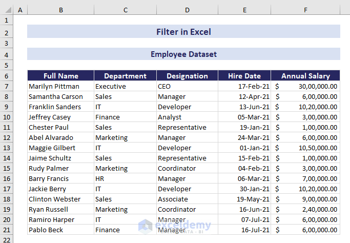
How to Add Filter in Excel
In this section, we will add Filter in Excel. We have a dataset that contains employee information about a company. Here, we have the employee’s name, department, designation, hire date, and salary. We want to add Filter to this data.
We can add Filter in Excel by following any of the three ways mentioned below:
– using the Home tab
– from the Data tab
– applying Keyboard shortcut
1. Add Filter in Excel Using Home Tab
If you want to add a filter to the header of the whole range of data,
- Select a random cell in the range or the whole range => navigate to the Home tab => Editing group => Sort & Filter drop-down => select Filter.
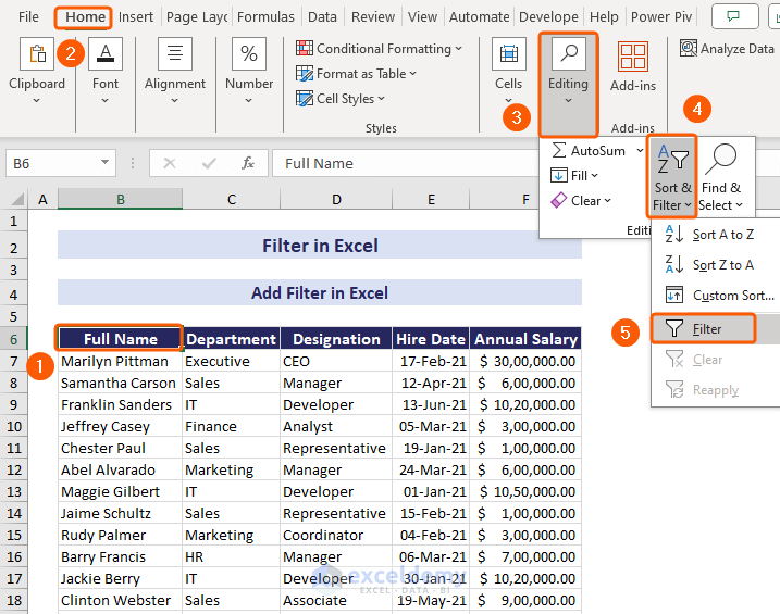
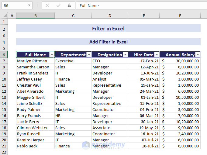
- It’ll add the filter button to the headers of the columns.
2. Insert Filter from Data Tab
Another way to add Filter in Excel is from the Data tab. This time we want to add Filter in the Department column only, not in the whole range.
- Select the range of cells in the Department column => navigate to the Data tab => and click on the Filter icon to add a Filter to the headers.
3. Applying Keyboard Shortcut to Add Filter
Excel also provides a way to enable the Filter with keyboard shortcut. Just select a cell in the range and press CTRL+SHIFT+L. Excel will add a Filter button to every column in the range.
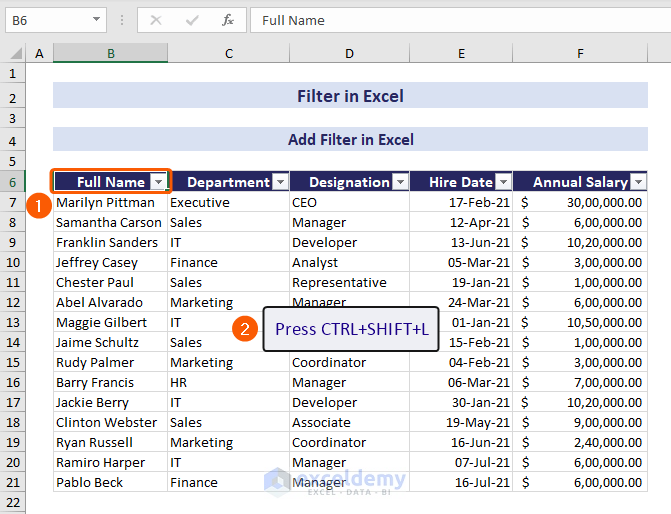
After enabling this feature, you can filter data based on cell value in Excel. For example, we can filter Manager from the Designation column following the GIF below.
How to Filter Data in Excel
You can filter data in Excel with the Filter feature according to your needs. For this purpose, Excel provides a number of ways:
– filter by text
– filter by number
– filter by date
– filter by search or partial match
– filter by cell color or text color
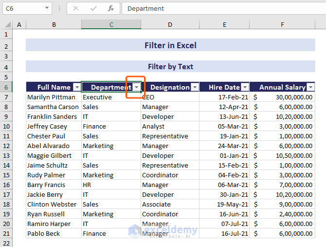
1. Filter by Text
For the dataset we have used previously, we want to filter data from the IT department. Here, we will use the Text Filter.
- Click on the drop-down arrow in the Department column.
- Click Text Filters => select Equals.
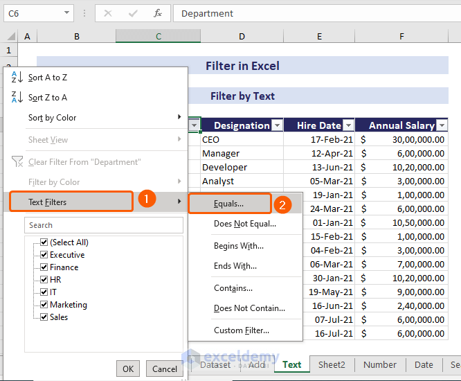
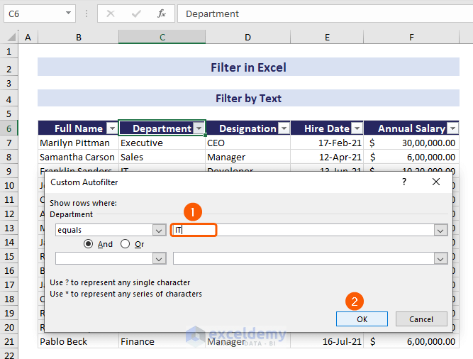
- This command launches the Custom Autofilter dialog box.
- As we want to filter data by the text “IT”, type IT right beside the equals field => click OK.
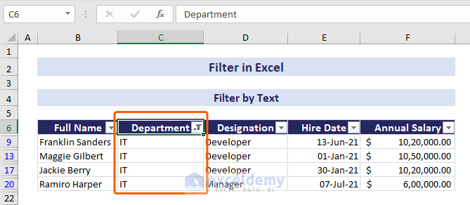
- Now, Excel makes only the relevant data visible to the IT department.
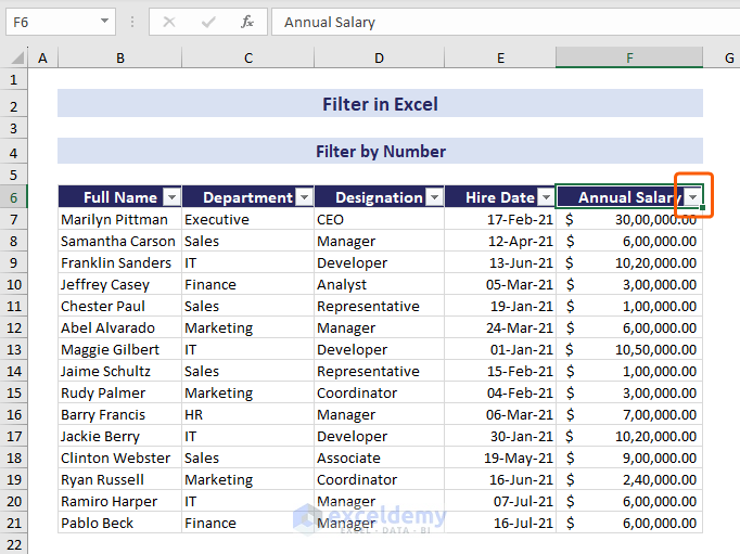
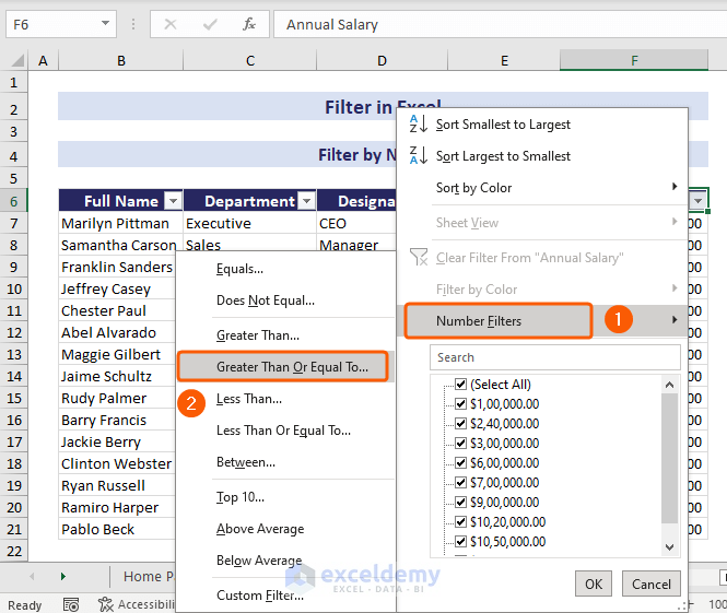
2. Filter by Number
Our dataset contains the annual salary of each employee. We want to filter the data of the employees whose salaries are more than or equal to $5,00,000. As this is a number, we will use the Number Filters for this task.
- Click the dropdown in the Annual Salary column.
- From the dropdown options, select Number Filers => click Greater Than Or Equal to.
- In the Custom Autofilter dialog box, type 500000 right beside the is greater than or equal field => and click OK.
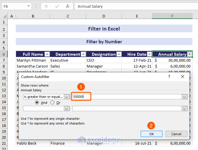
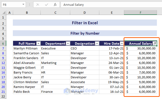
- This only filters the information of the employees about the given condition.
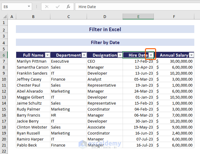
3. Filter by Date
Excel Date Filter feature allows you to filter data based on date values. You can group dates by filter in Excel. This feature provides several options, like filtering dates by month and year, filtering the last 30 days, etc.
Our dataset includes the Hire Date of the employees. We want to extract the information of the employees whose Hire Date is between 1 March 2023 and 31 March 2023.
- Click the dropdown in the Hire Date column.
- Click Date Filters and it will show a range of filter options for date => select Between. You can also select Custom Filter to use a custom date filter in Excel. Both of these commands will launch the Custom Autofilter dialog box.
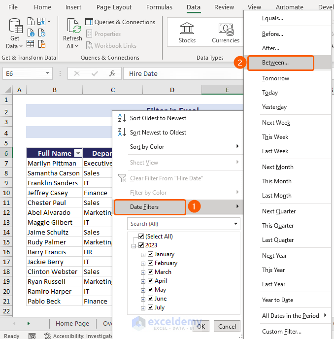
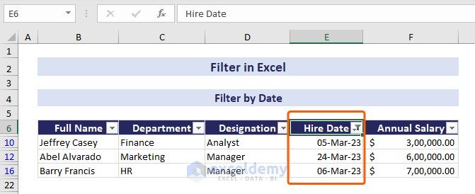
- In the is after or equal to field, type 1-Mar-23, and in the is before or equal to field, type 31-Mar-23 => click OK.
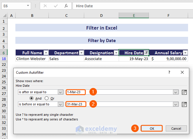
See! Excel has extracted only the data for the month of March.
4. Filter Data by Search or Partial Match
Instead of applying the built-in filter options, you can search for specific data and extract information with a partial match. From the Designation column of our dataset, we want to show the relevant data for the Coordinator role by searching for just the letters “Co” as a partial match.
- Click the drop-down in the Designation column.
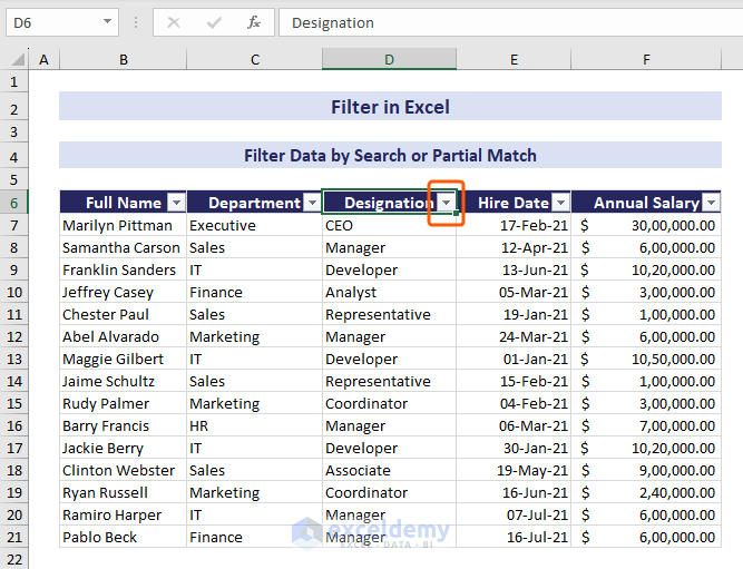
- In the search bar of the menu, type “Co” => click OK.
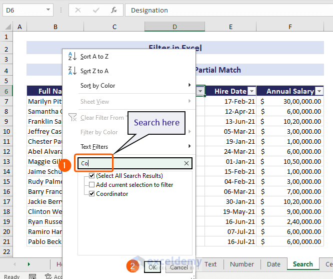
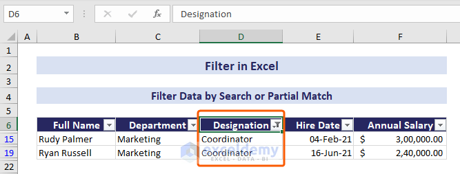
- Hence, it will match the relevant data whose first two letters start with “Co” which means “Coordinator” and show that data only.
5. Filter Data by Color
Color filter in Excel allows you to filter your data by color. You can filter your data
– Using cell color
– Using text color
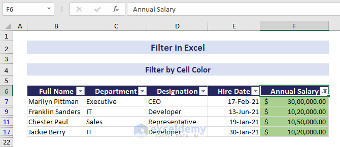
5.1. Filter by Cell Color
In the Annual Salary column of our dataset, we can see 3 colors in that cell range: green, yellow, and red. We want to filter data based on which cell color is green.
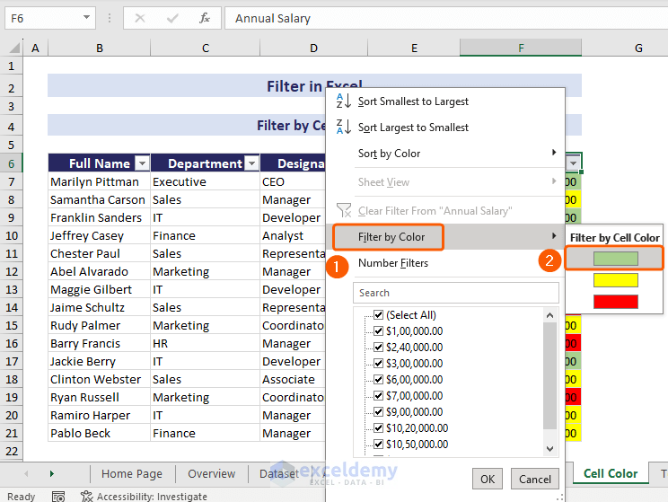
- Click on the filter button in the Annual Salary column.
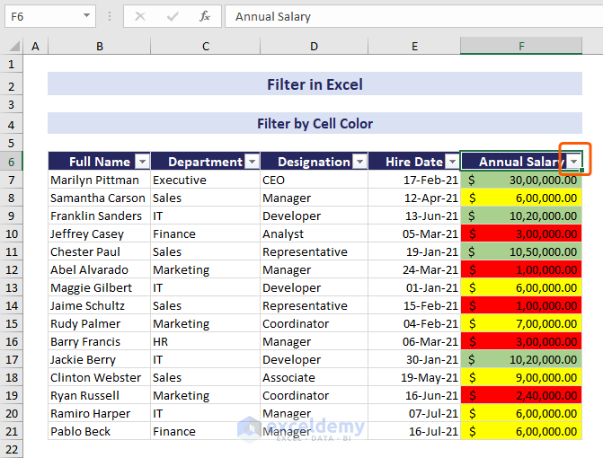
- Select the Filter by Color option in the menu bar => choose the Green color to filter by cell color.
- Now, Excel is only showing the filtered cells with the green color.
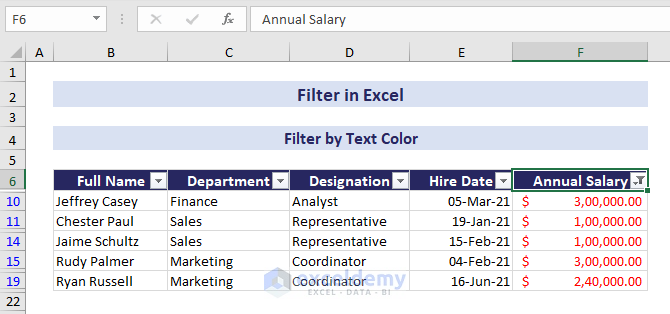
5.2. Filter by Text Color
This time, the Annual Salary column includes three text colors: green, blue, and red. We will choose green to filter by text color.
- Click on the Filter button in the Annual Salary column.
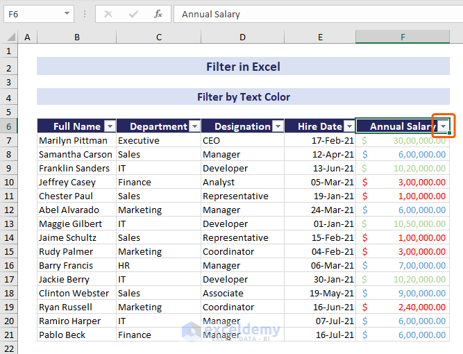
- Select the Filter by Color option in the menu bar => choose Red color to filter by text color.
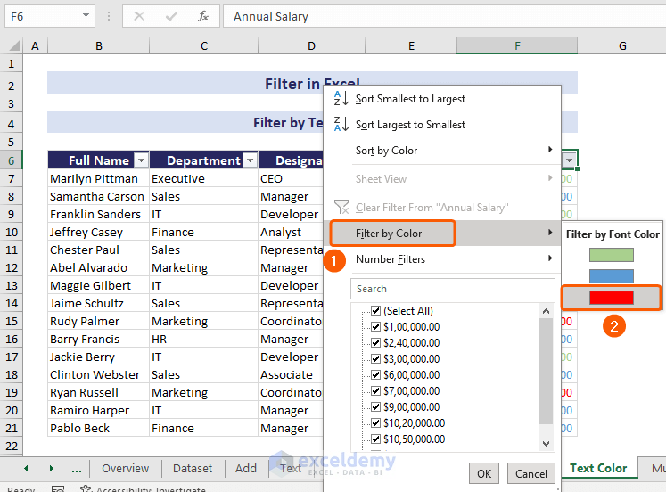
- See! Excel has filtered the data that only contain texts with red color.
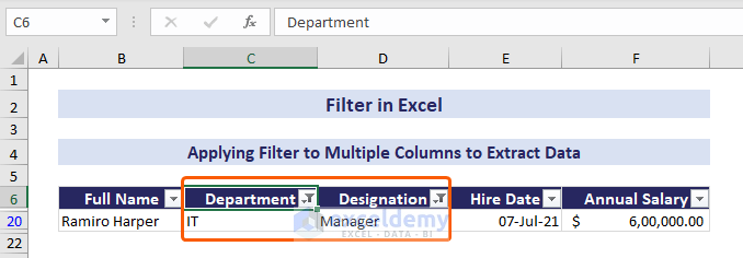
How to Apply Filter in Multiple Columns to Extract Data
In this section, we will filter one column based on another column in Excel. Considering multiple columns simultaneously helps to filter with multiple criteria. The dataset below contains employee information from different departments of a company. Each of the departments has several employees with different designations.
For example, the “IT” department has three “Developers” and one “Manager”. We will filter “Manager” information from the “IT” department. So we need to filter multiple columns simultaneously.
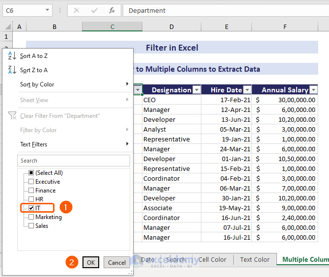
- First, click the dropdown in the Department column.
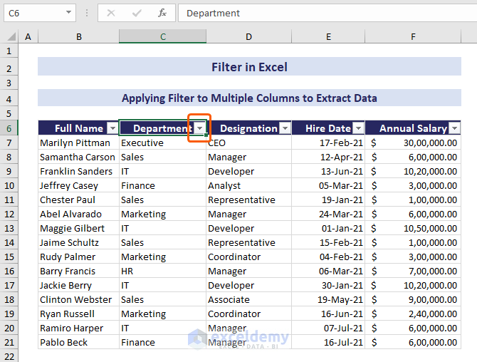
- Select IT from the filter options => click OK.
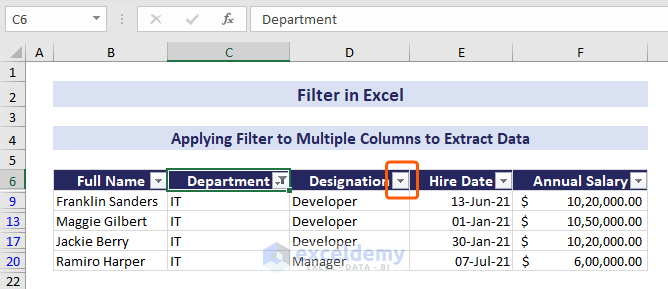
- Hence, the Department column will only show the cell values with IT.
- Now, click the drop-down in the Designation column.
- Select Manager => click OK.
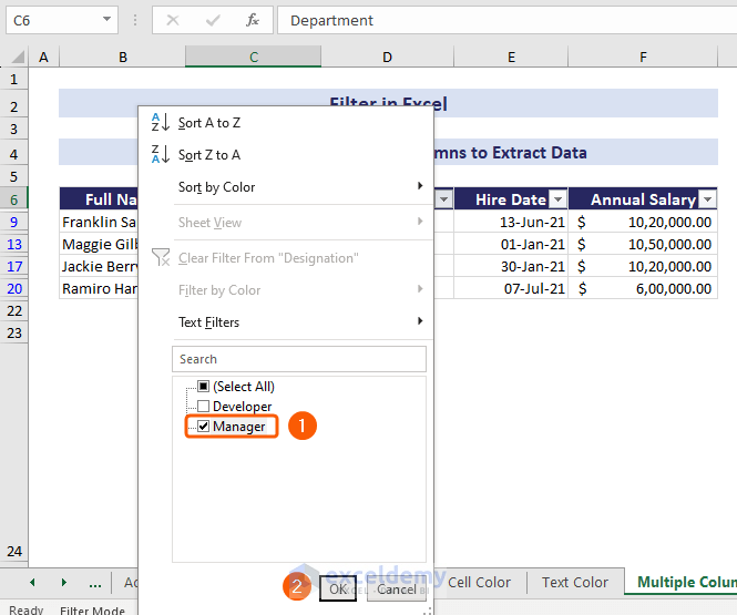
This time, Excel will show only the information of the Manager from the IT department.
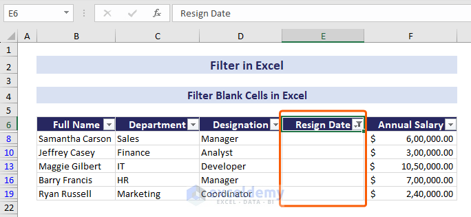
How to Filter Blank Cells in Excel
In this part, we will filter blank cells in Excel.
The dataset below has a column titled Resign Date. This column includes some blank cells corresponding to the employees who haven’t resigned yet and are still working. We want to show the data of the working employees.
- Click the dropdown of the Resign Date column.
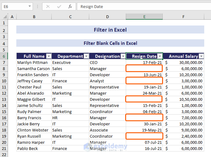
- From the dropdown options, keep the Blanks option selected only => click OK.
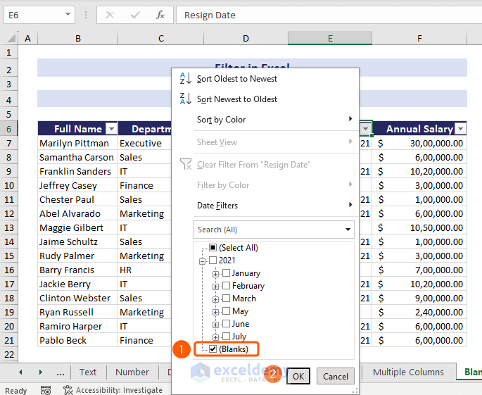
- Now, Excel is showing the rows with blank cells only and all the other rows are filtered out.
How to Use FILTER Function to Filter Data in Excel
In this segment, we will filter data in Excel using a formula. For this purpose, we will use the FILTER function.
The FILTER function filters a range or array in Excel. This function returns a dynamic result. When you change the values or array size of the source data, the results update automatically. This function is only available in Microsoft 365.
1. Filter Data Dynamically
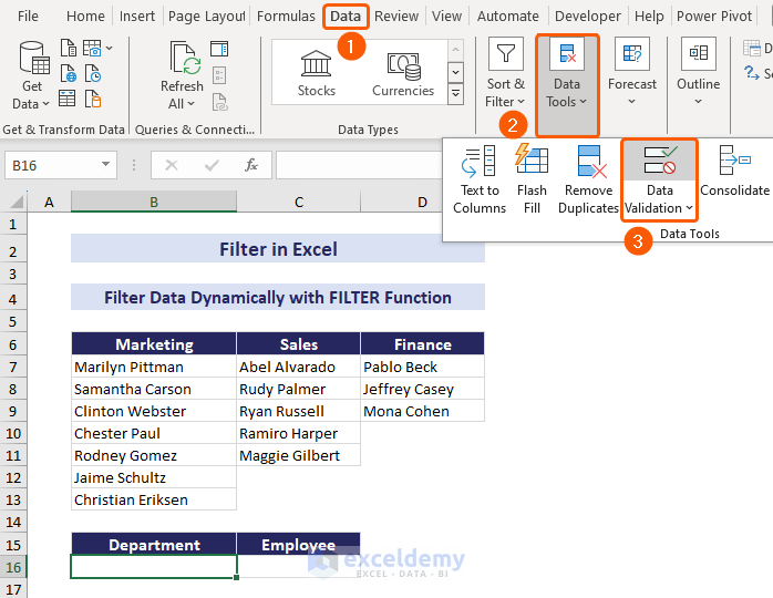
In this section, we will use the Excel drop-down list and FILTER function to filter data dynamically. The dataset below shows the employee names of three different departments: Marketing, Sales, and Finance. We will create a drop-down list for the department so that by choosing any department from the list, the employee names can be extracted dynamically with the FILTER function.
- Select cell B17 => go to the Data tab => Data Tools group => select the Data Validation feature.
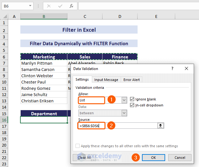
- This launches the Data Validation dialog box. In the Settings tab, choose List in the Allow field.
- In the Source field, select the list range or type:
=$B$6:$D$6- Click OK.
- Hence, you see a drop-down list.
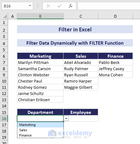
- Choose Marketing from the drop-down options.
- Now, select cell C16 => insert the following formula:
=FILTER(B7:D13,B16= B6:D6) & ""- Press ENTER. It will return all the employees of the selected department to cell B16.
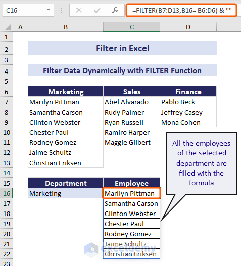
- Selecting a different value from the drop-down option in cell B16 will also change the output of the FILTER function in cell C16.
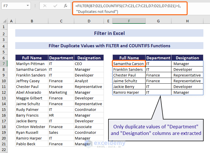
2. Filter Duplicate Values
If you want to filter only the duplicate values from the worksheet, you can do it by applying a combination of FILTER and COUNTIFS functions.
The dataset below shows an employee list with their corresponding designation and department. In the Department and Designation column, some values have occurred twice. Our aim is to show the duplicates. Using the COUNTIFS function, we will extract the data that occurred more than once.
- Select cell F7 => type the formula below.
=FILTER(B7:D21,COUNTIFS(C7:C21,C7:C21,D7:D21,D7:D21)>1,"Duplicates not found")- Press ENTER. You will get the duplicates that occurred in the Department and Designation column. If no duplicates were found, the formula would return “Duplicates not found”.
How to Use Advanced Filter in Excel
Like its name suggests, Excel Advanced Filter goes beyond the basic AutoFilter functionality. It provides more advanced criteria options. You will find this Advanced Filter feature in the Sort & Filter group. One of the basic differences between AutoFilter and Advanced Filter is that Advanced Filter allows you to copy the filtered results to another location, while AutoFilter doesn’t.
We will apply the Advanced Filter
– to find unique values
– for the wildcard character
– for multiple characters
– to exclude blank cells
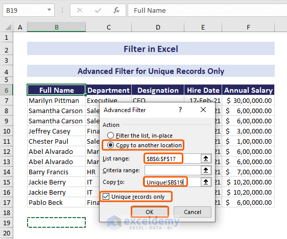
1. Find Unique Values in Worksheet
Let’s use the Excel Advanced Filter for unique records only. Our dataset has some duplicate values. From there, we will find the rows only with unique records with the Advanced Filter.
- Select a random cell in the range => go to the Data tab => click Advanced. It will launch the Advanced Filter dialog box.

- Keep Copy to another location marked.
- Fill the List range field by selecting your data range $B$6:$F$17.
- To fill in the Copy to field, select $B$19 in the worksheet where you want to copy the result.
- Put a checkmark on the Unique records only field.
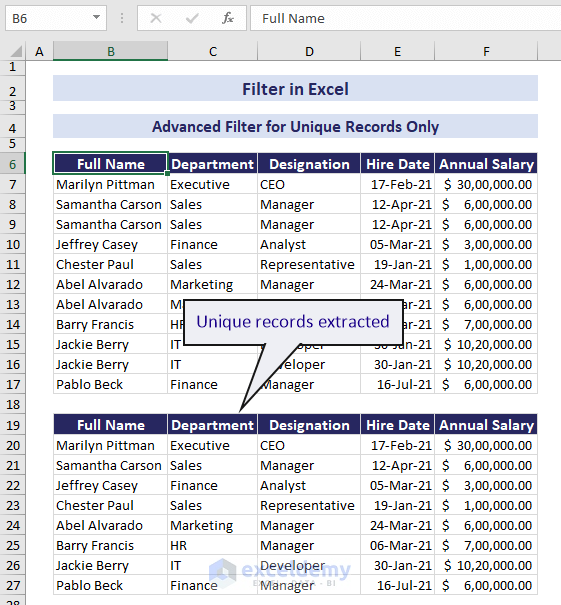
- Click OK.
You can see that Advanced Filter has extracted the unique records.
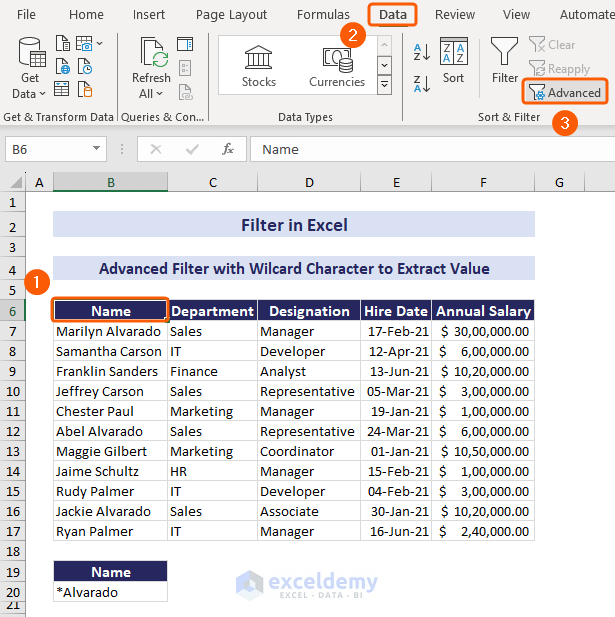
2. Advanced Filter with Wildcard Character to Extract Value
Now, we will use Advanced Filter with wildcard in Excel.
Wildcard characters like “asterisk” (*), “question mark” (?), and “tilde” (~) help with flexible and powerful searches. The (*) stands for any number of characters; (?) stands for one character; and (~) is used as an escape character.
The dataset below contains employee names where several people have common surnames. We will use “*Alvarado” to get all the information about employees whose surname is “Alvarado”.
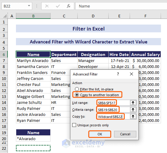
- Select a random cell in the range => go to the Data tab => and click Advanced to launch the Advanced Filter dialog box.
- Keep Copy to another location marked.
- Fill the List range field by selecting your data range $B$6:$F$17.
- Set the criteria range B$19:$B$20.
- To fill in the Copy to field, select $B$22 in the worksheet where you want to copy the result.
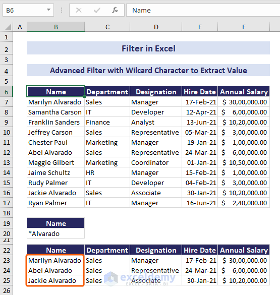
- Click OK.
Hence Excel has extracted the employee name, titled Alvarado.
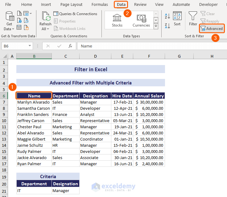
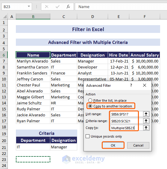
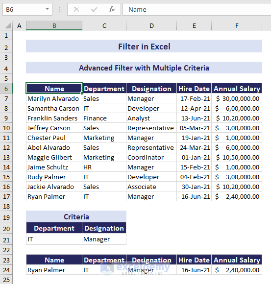
3. Advanced Filter with Multiple Criteria
At this stage, we will apply the Advanced Filter with multiple criteria in Excel. The dataset below contains employee information, where each department has several employees with different designations. We will filter Manager information from the IT department. So, our criteria are IT (department) and Manager (designation).
- Select a cell => go to the Data tab => and click Advanced to launch the Advanced Filter dialog box.
- Keep Copy to another location marked.
- Fill the List range field by selecting your data range $B$6:$F$17.
- Set the criteria range B$20:$C$21.
- To fill in the Copy to field, select $B$23 in the worksheet where you want to copy the result.
- Click OK.
So, Excel will extract the data of “Manager” from “IT” department.
Read More: Search Multiple Items in Excel Filter
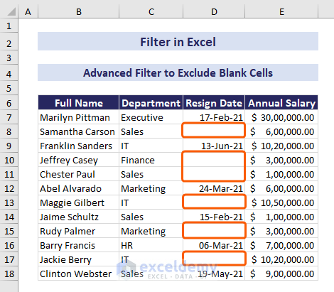
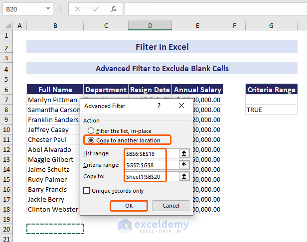
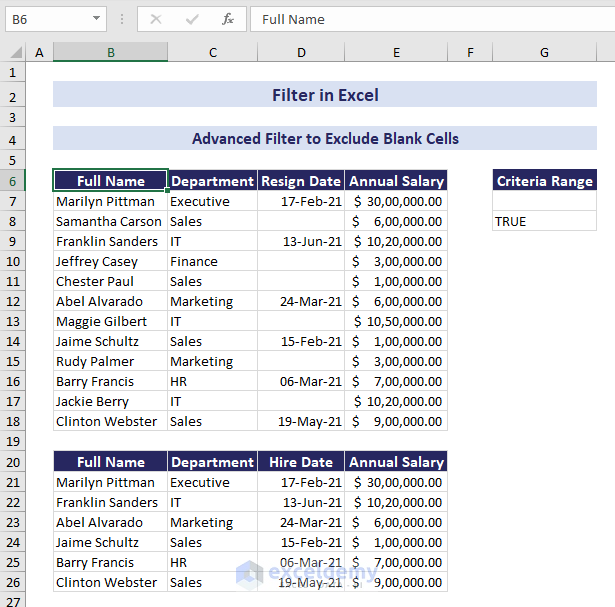
4. Advanced Filter to Exclude Blank Cells
We can also use the Excel Advanced Filter to exclude blank cells. Our dataset includes some blank cells, from which we want to exclude the rows with blanks.
- Insert the formula below in cell G8.
=D7<>"".- Press ENTER. It’ll return TRUE indicating that the value in cell D7 is not an empty string.
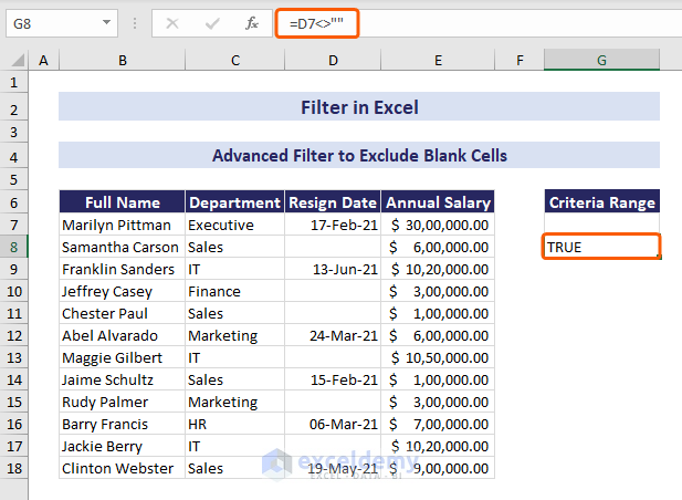
- Now, launch the Advanced Filter dialog box from the Data tab.
- Here, keep Copy to another location marked.
- Fill the List range field by selecting your data range $B$6:$E$18.
- Set the criteria range G$7:$G$8.
- To fill in the Copy to field, select $B$20 in the worksheet where you want to copy the result.
- Click OK.
You will get the result without the blank cells.
Read More: Use Filter in Protected Excel Sheet
How to Filter by Selected Icon or Format
Icon sets are a feature of conditional formatting that allows you to display icons (such as arrows, flags, or shapes) next to your data based on specific conditions. Icon sets are used to format cells to divide them into 3-5 groups from high to low values.
Our dataset shows the annual salary of some employees. The Annual Salary column is formatted with colored arrows, where green arrows show higher values. We will filter the data based on the green arrows.
![]()
- Select cell F7 formatted with the green arrow => right-click to bring up the context menu.
- Select Filter => click Filter by Selected Cell’s Icon.
![]()
- Hence, Excel will filter your data according to the format you selected in the first step.
![]()
Read More: Filter with Multiple Criteria in Excel
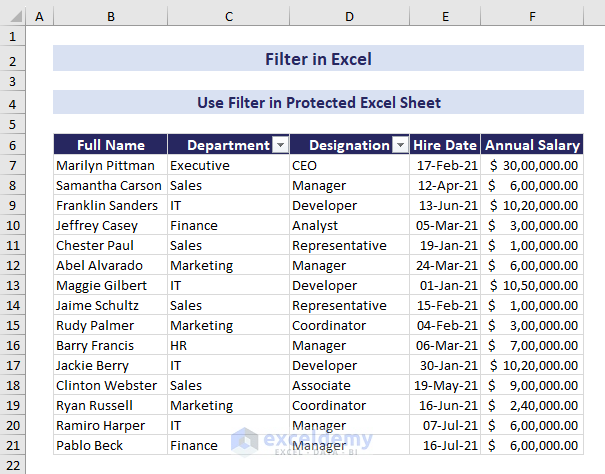
How to Use Filter in Protected Excel Sheet
Excel allows you to use Filter in a protected Excel sheet.
For the dataset below, we have enabled Filter in the Department and Designation columns. We will use this filter on a protected worksheet.
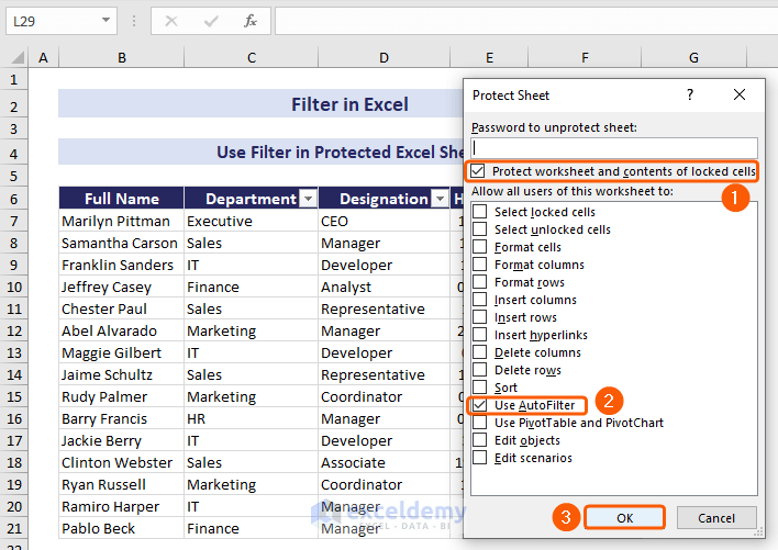
- To protect the worksheet, go to the Review tab => and click Protect Sheet to launch the Protect Sheet dialog box.
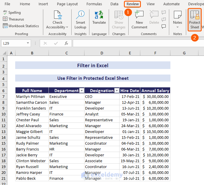
- Keep the Protect worksheet and contents of locked cells marked.
- Mark Use AutoFilter option only => click OK.
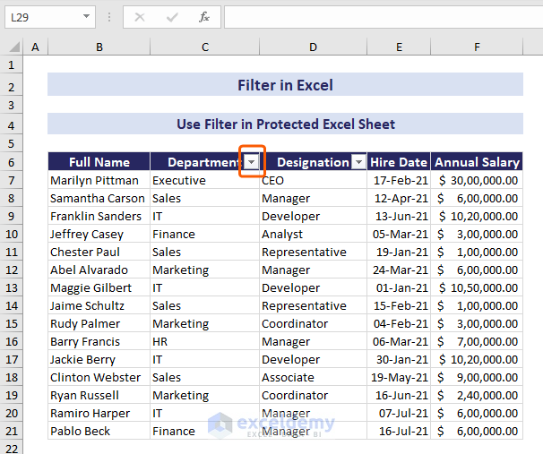
Your worksheet is now protected. You won’t be able to select any cells. But you have access to the Filter button.
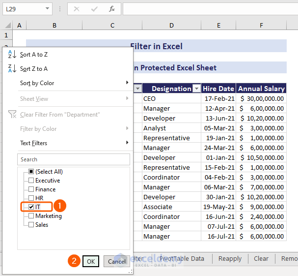
- Click the drop-down in the Department column.
- Select IT => click OK.
Although you can’t select or edit any cell, Excel allows you to filter data in a protected sheet in this way.
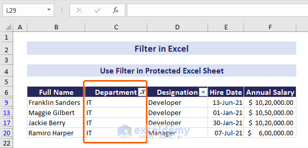
You can also filter the Designation column similarly. But you won’t be able to filter other columns.
Read More: Convert Text Filter to Date Filter in Excel
How to Filter Data in Excel Pivot Table
In this section, we’ll filter the data in the Pivot Table. The dataset below shows sales reports of some products in different states with their quantity and sales amount.
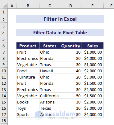
We will create a Pivot Table with this data and then filter the data in that Pivot Table.
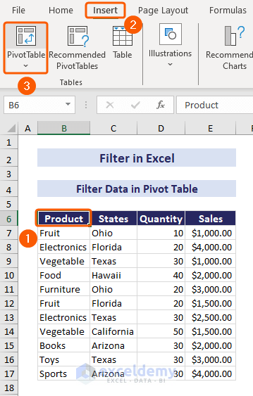
- Select any cell in the range => go to the Insert tab => select PivotTable.
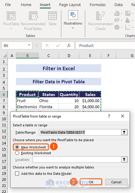
- The PivotTable from table or range dialog box will appear. Choose New Worksheet to place the PivotTable => click OK.
Excel will take you to a new worksheet. The PivotTable Fields pane will appear on the right side of that new worksheet.
- Insert the parameters in the following field:
– Filters: States
– Rows: Product
– Values: Quantity and Sales
As a result, Excel will create the Pivot Table.
- Now, select a cell in the PivotTable => go to the PivotTable Analyze tab => and click Insert Slicer.
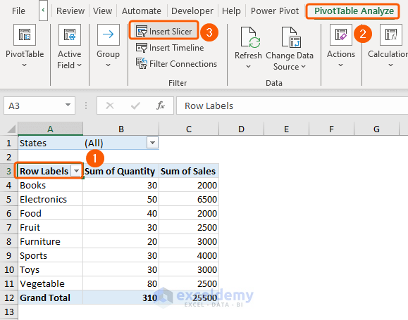
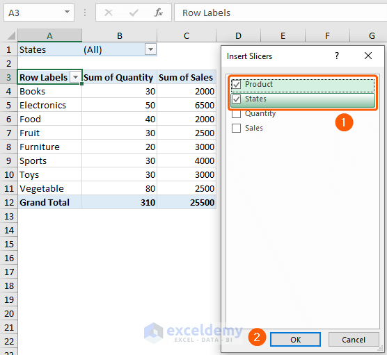
- In the Insert Slicers dialog box, select Product and States => click OK.
- This will insert two slicers titled Product and States.
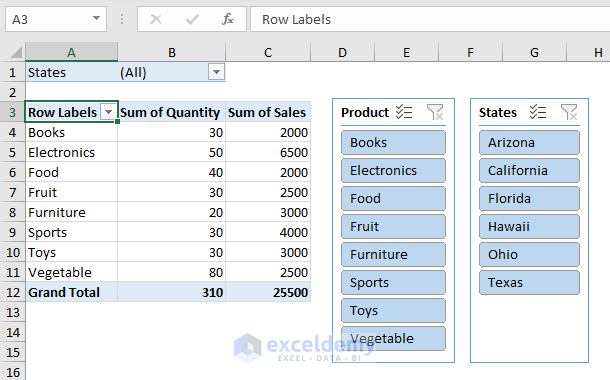
- Select any item in the Product Slicer, and you will see that the States slicer is automatically showing the state where the product is available. In the meantime, the Pivot Table will show the price of that product.
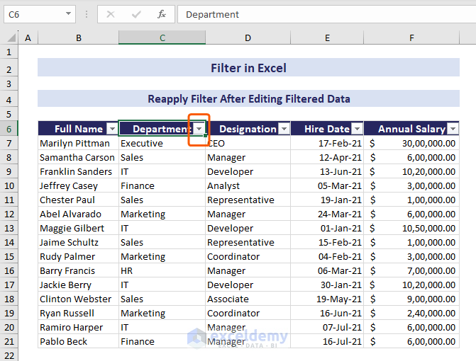
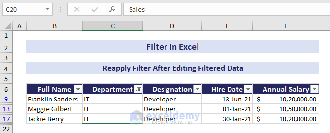
How to Reapply Filter After Editing Data in Excel
After applying Filter, if you change or modify any filtered data, Excel doesn’t automatically update the edited data. You have to reapply Filter to show the change.
- First, filter the department column by “IT” as we have done previously.
- Change a filtered cell from “IT” to “Sales”.
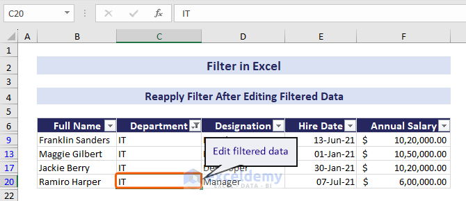
- You will see the Filter is not updating the list.
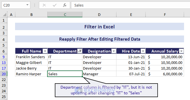
- To update the list, go to the Data tab => Sort & Filter group => click Reapply.
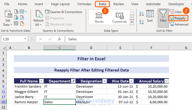
Now, you will see the updated filtered data.
How to Clear Filter in Excel
To undo or clear filtered items from the Department column to make all the data visible again,
- Click on the Filter button to bring up the filter options.
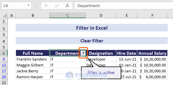
- Select Clear Filter from “Department” option.
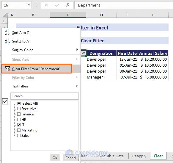
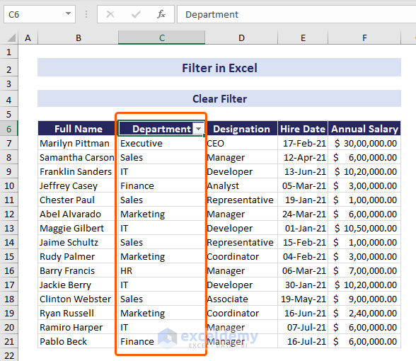
- It will make the Filter inactive and show all of the data again.
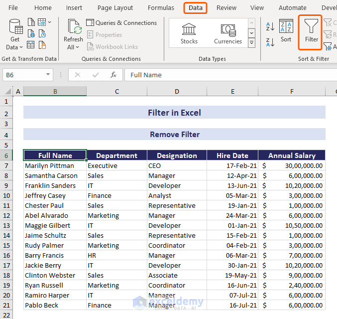
How to Remove Filter in Excel
You may need to remove Filter in Excel to show your data like the original one.
- Navigate to the Data tab => Sort & Filter group => click on the Filter icon to deactivate it.
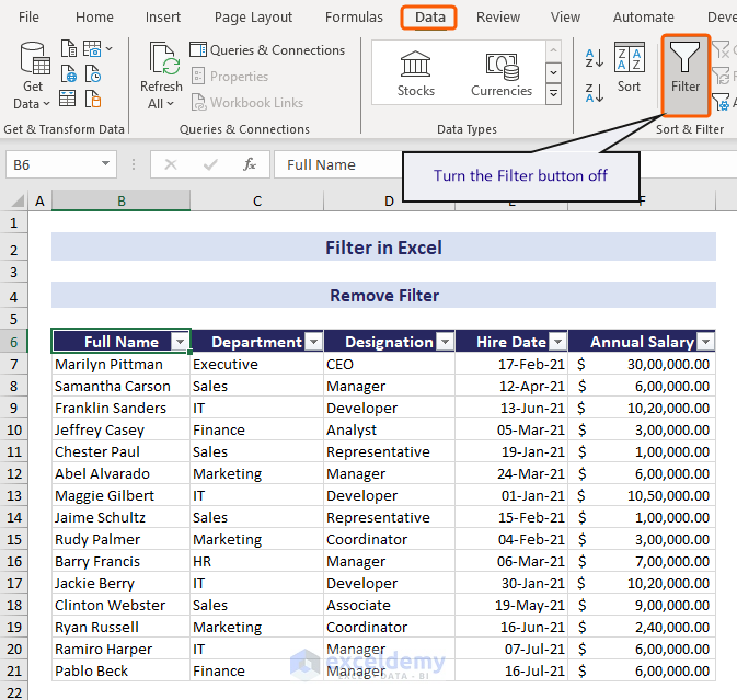
With the deactivation, Excel will remove the Filter button from your data.
How to Fix If Filter Is Not Working in Excel
Sometimes you may face some problems, like the Excel filter not working after a certain row or not filtering the entire column. This may occur for several reasons.
- If your data range includes blank rows, then you may face a problem because the Excel filter stops at blank row. In this case, select your data range manually before applying Filter. You can also Sort your data in ascending order and then apply the Filter command.
- When Excel doesn’t update after any change in filtered data, just use the Reapply command.
- Merged cells can interfere with the functioning of filters. If merging is necessary, then learn to filter in Excel with merged cells.
- If there are variations in cell formats (such as text mixed with numbers), Excel might have difficulty applying filters. Ensure that all data in the filtered range is formatted consistently.
What Is the Difference Between Sort and Filter in Excel
The Sort feature allows you to organize and arrange the data in your worksheet in a specific order based on one or more criteria. However, the Filter feature only allows the showing of data based on criteria.
To apply the Sort feature:
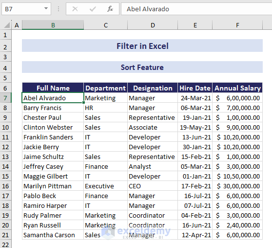
- Select a cell in the column you want to sort => Data tab => click Sort A to Z.
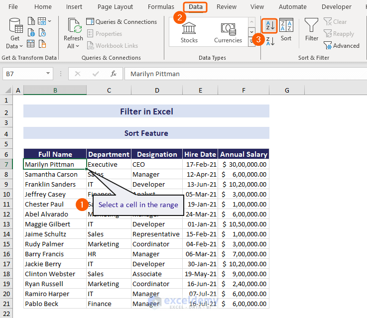
It will expand the selection and sort your data in alphabetically ascending order.
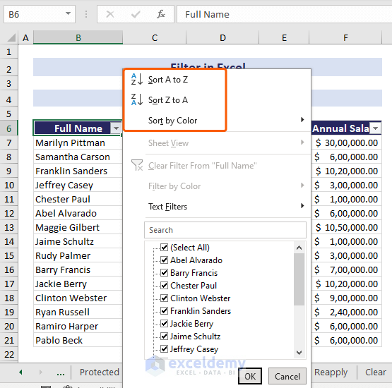
However, you can also access the Sort feature from the Filter drop-down options.
Download Practice Workbook
In this article, we have learned to add Filter in Excel and filter our data by text, number, date, search, and color. We have also learned different methods to apply the Filter, such as filtering multiple columns, blank cells, selected icons, and pivot tables. Moreover, we discussed the FILTER function and the Advanced Filter feature. Further, it showed how to clear the filtered data and remove the Filter in Excel.
Filter in Excel: Knowledge Hub
<< Go Back to Learn Excel

