Here, we will learn Excel compare columns using different processes and formulas such as conditional formatting, IF function, EXACT function, AND function. We will use all possible functions as well as different procedures.
Comparing columns is a very basic yet vital feature. We can get the duplicate and unique values by comparing two columns. Comparing columns creates data cleansing, deletes differences, analyzes the data, and returns the proper result. If you compare columns, then you can identify the matches and sort the data according to the match, making the dataset more readable and more presentable as well.
The overview of this article is shown below. You may follow the whole article to get proper information about excel compare columns.
How to Compare Columns in Excel: 9 Methods
To compare columns in Excel here we will use different procedures and formulas.
Method 1: Comparing Two Columns in the Same Row
In this method, we will use the IF function to compare two columns. here is the overview image of the IF function below. Click on the image to get a proper visualization.

- If the value in column C matches the value in column D, then the formula will return the value as Matched.
=IF(C5=D5,"Matched","Not Matched")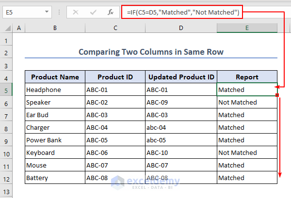
Method 2: Using EXACT Function to Compare Upper/Lower Case Data in Columns
The previous method returns output if the value matches, but sometimes values are not the same when they’re written in a different case. Here we will use the EXACT function to differentiate and compare upper case or lower case data.
- Now, select cell E5 and enter the below formula.
=IF(EXACT(C5,D5),"Matched","Not Matched")
Formula Breakdown
EXACT(C5,D5)
- This function returns the exact value of the cells.
IF(EXACT(C5,D5),”Matched”,”Not Matched”)
- Here, if the columns match the value with the same case, then this formula returns the value as “Matched” otherwise “Not Matched”.
Method 3: Comparing Multiple Columns in Same Row
Here we will use the IF and AND functions to compare multiple columns in the same row.
- Insert the formula in cell F5 and compare the data in multiple columns.
=IF(AND(C5=D5, C5=E5), "Full match", "Not Matched")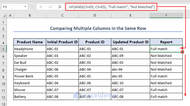
Formula Breakdown
AND(C5=D5, C5=E5)
- The AND function adds the value if there are more than two values.
IF(AND(C5=D5, C5=E5), “Full match”, “Not Matched”)
- Here, the formula will return the value if all the columns match the value; otherwise “Not Matched”.
Read More: How to Compare Two Columns or Lists in Excel
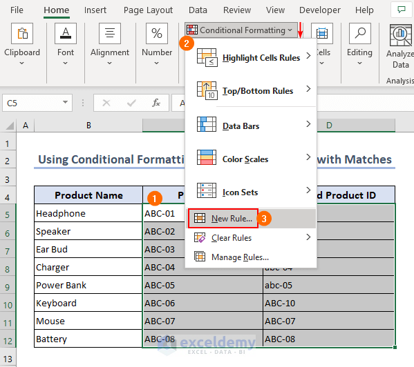
Method 4: Using Conditional Formatting to Compare Columns with Matches and Mismatches
Here, we will use conditional formatting to compare the matches and then highlight the matches with suitable colors.
- In the beginning, select range C5:D12 and click on Conditional Formatting from the toolbar.
- The drop-down option will pop up, and select New Rule from the list.
- Edit Formatting Rule dialog box will pop up. and select Use a formula to determine which cells to format, write down the formula, and click OK.
=$D5=$C5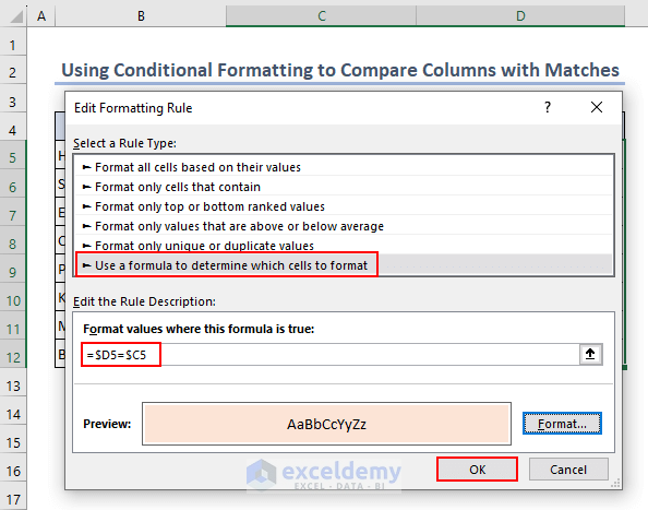
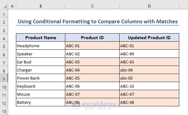
- The final output will be below.
- Now, we will compare the mismatches in the columns. All the Procedures will be the same, but the formula.
=$D5<>$C5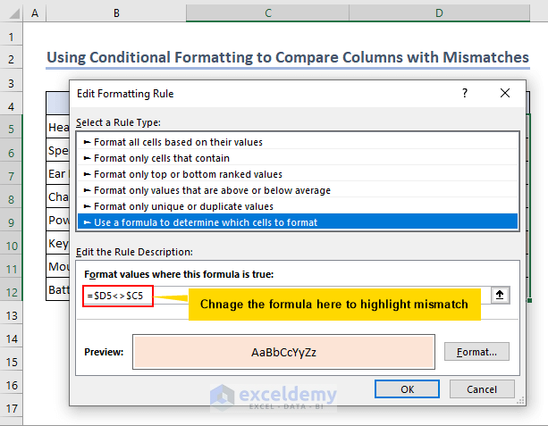
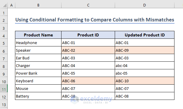
- Lastly, the final output will be similar to below.
Read More: Excel Formula to Compare and Return Value from Two Columns
Method 5: Combining IF and COUNTIF Functions to Compare Two Columns
Here, we will combine the IF function and the COUNTIF function to compare two columns. Initially, select cell E5 and enter the formula.
- Therefore, apply the formula in cell E5 as below.
=IF(COUNTIF($D:$D, $C5)=0, "No match in D", "Match")
Formula Breakdown
COUNTIF($D:$D, $C5)=0
- This part returns the value as true or false. The COUNTIF function counts the matches.
IF(COUNTIF($D:$D, $C5)=0, “No match in D”, “Match”)
- This formula returns the value if there is a match in columns C and D; otherwise, it returns the value “No match in D.
Read More: How to Compare Two Lists and Return Differences in Excel
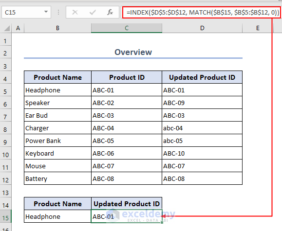
Method 6: Combining INDEX MATCH Functions to Pull Matches from Two Lists
The INDEX function and the MATCH function pull out the matches and return the value of the corresponding lookup value.
- Enter the formula in cell B15 and execute this process.
=INDEX($D$5:$D$12, MATCH($B$15, $B$5:$B$12, 0))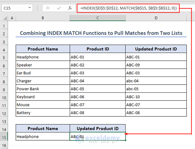
Formula Breakdown
INDEX($D$5:$D$12)
- The INDEX function returns the result value here.
INDEX($D$5:$D$12, MATCH($B$15, $B$5:$B$12, 0))
- Here, the lookup value is in cell B15, and if the value matches column B, then this formula will return the corresponding value from column D.
Read More: How to Match Two Columns and Return a Third in Excel
Method 7: Utilizing VLOOKUP Function to Compare Values from Columns
The VLOOKUP function matches the range with the lookup value, and here is the overview image of the VLOOKUP function. Click the image for better visualization.

- Now, the lookup value in cell B15 matches the lookup range, then the formula returns the corresponding value of the column.
=VLOOKUP(B15,$B$5:$D$12,3,0)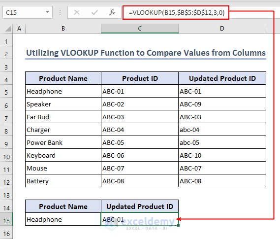
Read More: Comparing Two Columns and Returning Common Values in Excel
Method 8: Combining IF and MATCH Functions to Compare Two Columns
Here we will apply the IF function, the ISERROR function, and the MATCH function to compare two columns.
- Select cell E5 to execute this process.
=IF(ISERROR(MATCH( $C5,$D:$D,0)), "No match in D", "Match")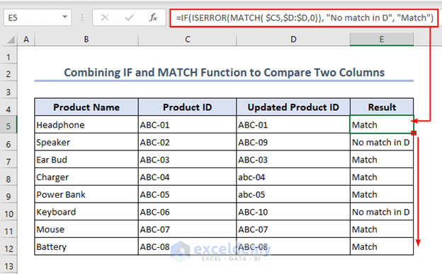
Formula Breakdown
MATCH( $C5,$D:$D,0)
- This part searches the value of cell C5 in column D for an exact match.
(ISERROR(MATCH( $C5,$D:$D,0))
- This part returns the value as True if there is any error; otherwise, it is false.
IF(ISERROR(MATCH( $C5,$D:$D,0)), “No match in D”, “Match”)
- The formula will search the value of cell C5 in column D and returns the value as “Match” if there is any match; otherwise, “No Match in D”
Method 9: Comparing Two Columns in Excel and Counting Matches
In this method, we will use the SUMPRODUCT function to compare the columns and count the matches. Here is the overview image of the SUMPRODUCT function is below. click on the image to get better visualization.
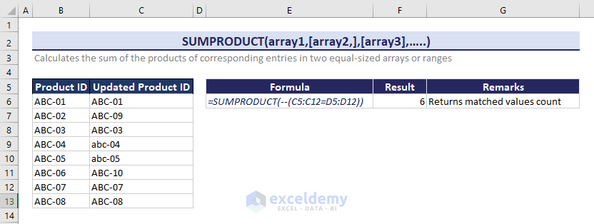
- This formula will count the matches in the ranges C5:C12 and D5:D12.
=SUMPRODUCT(--(C5:C12=D5:D12))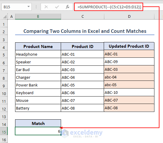
Read More: How to Compare Text in Two Columns in Excel
How to Compare Rows in Excel: 2 Methods
To compare rows in Excel here, the column will be the same and the rows will be different.
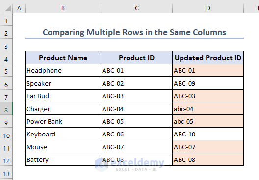
Method 1: Comparing Multiple Rows in Same Columns
In this method, we will compare and highlight the rows in the same columns using Conditional Formatting.
- This process is similar to before, but the formula has changed. Insert the below formula to execute this process.
=COUNTIF($D$5:$D12,C5)>0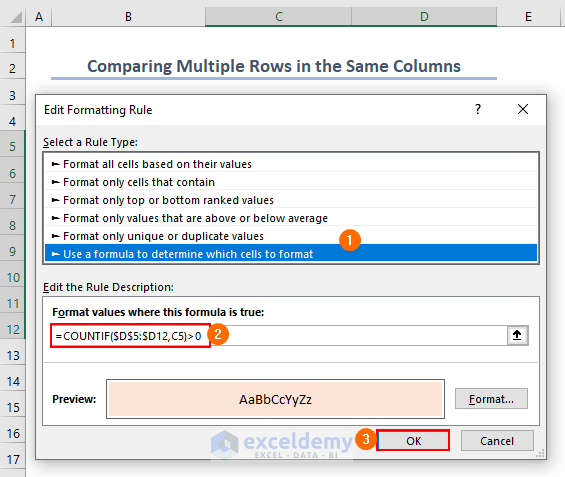
- Here is the final output after completing the process.
Method 2: Using the IF Function to Compare Multiple Rows in the Same Column
In this method, we will use the SUM function and the IF function to get the sum of the matches in column D.
- Select cell B15 and execute the process.
=SUM(IF(D5:$D$12= D5, 1, 0))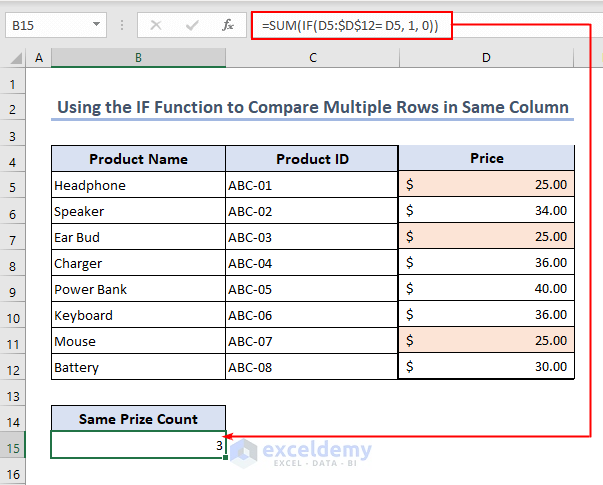
Formula Breakdown
IF(D5:$D$12= D5, 1, 0)
- This part returns the count of matched values in column D.
SUM(IF(D5:$D$12= D5, 1, 0))
- This formula will return the sum of the matched value counts in column D.
Things to Remember
- Make sure that the columns you are comparing contain the same type of data. For instance, both columns should contain Text or Numbers.
- Sometimes case sensitivity is important, so use the EXACT function if the output needs to be case sensitive.
Download Practice Workbook
You may download the workbook for practice.
Conclusion
In this article, we learned how to perform Excel compare columns using different processes and formulas. Here, we also learned how to compare rows in the same column. We covered every possible aspect of this process. Hopefully, you can solve the problem shown in this article. Please let us know in the comment section if there are any queries or suggestions, or you can also visit Exceldemy to explore more.
Frequently Asked Questions
Q1: How do I compare two Excel lists for matches?
Ans: First, select the lists and go to Conditional Formatting >> Duplicate Values >> OK.
Q2: How can I compare 3 columns in Excel?
Ans: If you want to compare three columns, then use this formula- =IF(AND(C1=C2, C1=C3), “Full match”, “Not Matched”)
Q3: How can I compare columns in different sheets?
Ans: To compare columns in different sheets follow the formula here Sheet1!B5=Sheet2!B5.
Excel Compare Columns: Knowledge Hub
- Compare 3 Columns for Matches in Excel
- Compare Three Columns and Return a Value
- Compare Three Columns Using VLOOKUP
- Compare Two Columns Using VLOOKUP Function
- VLOOKUP Formula to Compare Two Columns in Different Sheets
- How to Compare 4 Columns in Excel
- How to Compare 4 Columns in Excel VLOOKUP
- Match Multiple Columns in Excel
<< Go Back to Compare | Learn Excel

