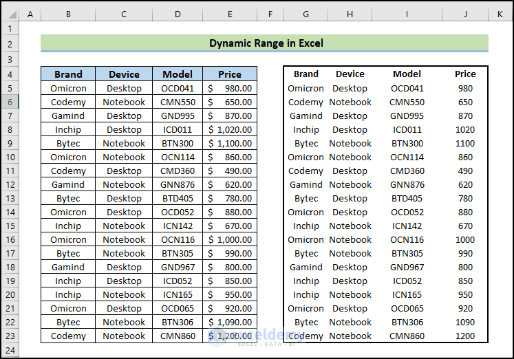
Excel Dynamic Range (Complete Guideline)

Get FREE Advanced Excel Exercises with Solutions!

In this article, we will demonstrate how to create a dynamic range in Excel.

We will go over topics including defining dynamic ranges, using dynamic range references in formulas, and applying dynamic ranges to charting. To increase the functionality of dynamic ranges, we will also demonstrate techniques, such as named ranges and array formulas.

To save them time and effort, you will learn how to create formulas and references that automatically adapt as data is added, deleted, or changed.

Download Practice Workbook

Download this practice workbook to exercise while you are reading this article.

Dynamic Range.xlsx

Table of Contents Expand

How to Create a Dynamic Named Range in Excel

1. INDEX Formula to Make a Dynamic Named Range in Excel

Here, we will create an INDEX formula to create a dynamic chart range.

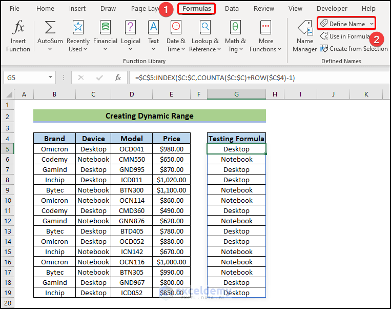
Write down the following formula in cell G5.

=$C$5:INDEX($C:$C,COUNTA($C:$C)+ROW($C$4)-1)

To use the dynamic range in a formula later, create a named range. Select and copy the formula from cell G5, go to the Formulas tab, and click on the Define Name button.

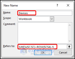
The New Name window will appear. Give a suitable name to the range (Devices here).
Paste the copied formula in the Refers to: box and press OK.

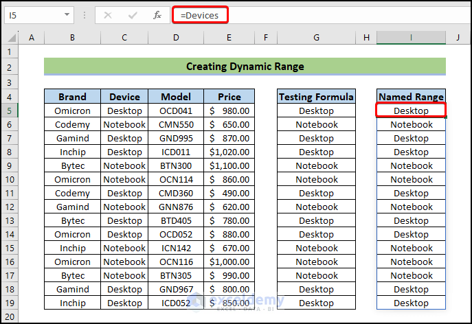
Now, we will apply the dynamic named range and test If it is created properly.
Select a cell and write down the following formula.

=Devices

By inserting a new device in column C, you may determine whether or not everything is operating as it should.

2. OFFSET Formula to Define an Excel Dynamic Named Range

The OFFSET function is another option to create dynamic ranges in Excel.

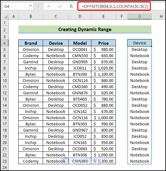
To get 1 column (Device column) dynamic range, use the following formula.

=OFFSET($B$4,0,1,COUNTA($C:$C))

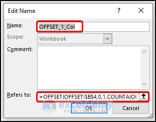
You can also make a dynamic range by creating a named range. Select and copy the formula from cell G5, go to the Formulas tab, and click on the Define Name button.
The New Name window will appear. Give a suitable name to the range
Paste the copied formula in the Refers to: box and press OK.

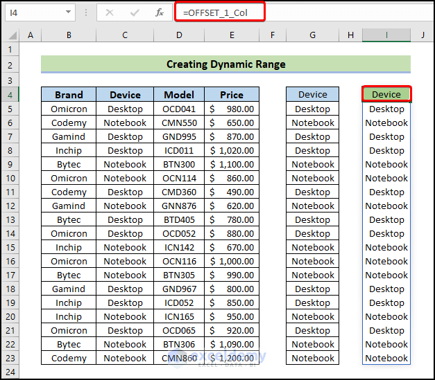
Now, we will apply the dynamic named range and test If it is created properly.
Select a cell and write down the following formula.

=OFFSET_1_Col

You can check to see if everything is working properly by adding a new device to column C.

Dynamic Range for Multiple Columns in Excel

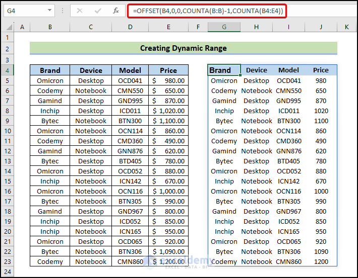
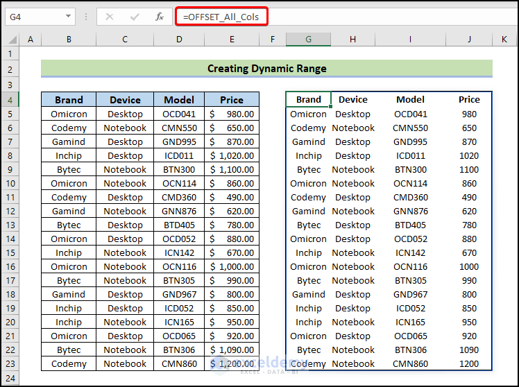
To get multiple columns dynamic range (starts from cell B4, covers columns B to E, and so on), apply the following formula.

=OFFSET(B4,0,0,COUNTA(B:B)-1,COUNTA(B4:E4))

Now, when you add any item in columns B and E, you will see the corresponding change in the dynamic range you have created.

You can also make a dynamic range for multiple columns by creating a named range. Go to the Formulas tab, and click on the Define Name button.
The New Name window will appear. Give a suitable name to the range
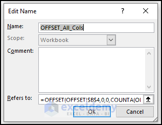
Type the following formula in the Refers to: box and press OK.

=OFFSET($B$4,0,0,COUNTA($B:$B)-1,COUNTA($4:$4))

We will now use the dynamic named range to see if it was correctly created.
Select a cell and write down the following formula.

=OFFSET_All_Cols

By adding a new device to column C, you can verify that everything is operating as it should.

Pros and Cons of Dynamic Range in Excel

In Excel, dynamic range refers to the ability to automatically adjust the range of cells included in a formula or data analysis as new data is added or existing data is modified.

Pros of using a dynamic range in Excel:

You can work with changing data sets without manually updating formulas or analysis ranges by using a dynamic range.
You can save time by eliminating the need to modify formulas whenever new data is added by using dynamic range references.
Dynamic ranges reduce the possibility of errors that can occur when manually updating ranges.

Cons of dynamic range in Excel:

It can be more difficult to implement dynamic range formulas than fixed ranges. It necessitates an understanding of sophisticated techniques like named ranges, OFFSET, INDEX, or structured references, which may call for further education or experience.

Things to Remember

When you create a named range, use an absolute reference. Otherwise, when you move the placement to another cell, Excel will alter the formula’s cell references, resulting in incorrect output.
In the Refers to: box, press the F2 key to make the right or left arrow keys work.

Conclusion

In conclusion, the dynamic range of Excel is an effective feature that enables the development of adaptable and automatic formulas.

When referring to a dynamic range of cells, you can indicate a set of cells that changes as new data is added or removed automatically. The efficiency, accuracy, and adaptability of data analysis, reporting, and visualization tasks are improved by dynamic ranges.

Overall, becoming proficient in Excel’s use of dynamic ranges can increase productivity significantly and give users the ability to handle data-driven tasks with ease.

Frequently Asked Questions

1. What are some common scenarios where dynamic range is useful in Excel?

Dynamic range is useful in various scenarios, such as performing calculations on fluctuating data, creating charts or graphs that update automatically, working with pivot tables, and simplifying data analysis by eliminating the need for manual updates when new data is added.

2. Can I use dynamic range with formulas in Excel?

Yes, dynamic ranges can be used with formulas in Excel. Formulas can reference dynamic ranges to perform calculations on changing data automatically.

3. How do I update a dynamic range when new data is added?

The dynamic ranges in Excel update automatically when new data is added or existing data is modified, thanks to the dynamic ranges formulas used to define the ranges.

Excel Dynamic Range: Knowledge Hub

<< Go Back to Excel Named Range | Excel Formulas | Learn Excel