When you open an Excel workbook, the grid-like faint gray lines presenting the cells, rows, and columns are formally known as Excel Gridlines.
In this Excel tutorial, you will learn all about Excel gridlines.
By default, Excel worksheets have gridlines. However, if you want to work on a blank sheet, without gridlines, you can simply turn it off.

In this article, you will learn how to
– Show gridlines on a worksheet
– Turn off gridlines
– Show gridlines for specific cells
– Hide gridlines for specific cells
– Remove gridlines from multiple worksheets
– Change the color of Excel gridlines
– Show gridlines after using fill color
– Print gridlines on a worksheet
Gridlines in Excel provide a visual guide to users that helps to navigate and organize data on a worksheet. This, in turn, enhances the readability and overall structure of the spreadsheet. Users in truth often take the help of gridlines for aligning and arranging content.
⏷ What Are Gridlines?
⏷ How to Show Gridlines on a Worksheet
⏷ How to Turn Off Gridlines
⏷ Hide Gridlines in Excel Without Turning Off
⏷ Showing Gridlines for Specific Cells
⏷ How to Hide Gridlines for Specific Cells
⏷ Removing Gridlines from Multiple Worksheets
⏷ How to Change the Color of Gridlines
⏷ Showing Gridlines After Using Fill Color
⏷ Print Gridlines on a Worksheet
What Are Gridlines in Excel?
Gridlines in Excel are the faint, gray lines that separate and define cells within a worksheet. These lines serve as visual guides, helping users distinguish the cells, rows, and columns.
Gridlines are visible across the entire worksheet and cannot be applied to a specific region. By default, gridlines are not shown when you print an Excel sheet. However, you can turn on gridlines on Page Setup and show them in printed Excel sheets.
You can find gridline settings in the Advanced menu of Excel Options, Page Layout tab, and View Tab.
How to Show Gridlines on a Worksheet in Excel?
You can show the gridlines on a worksheet in Excel by turning on the Gridlines option from the View or Page Layout tab and from the ‘Display options for this worksheet’ menu of Excel advanced options.
Besides, you can use a keyboard shortcut to show gridlines.
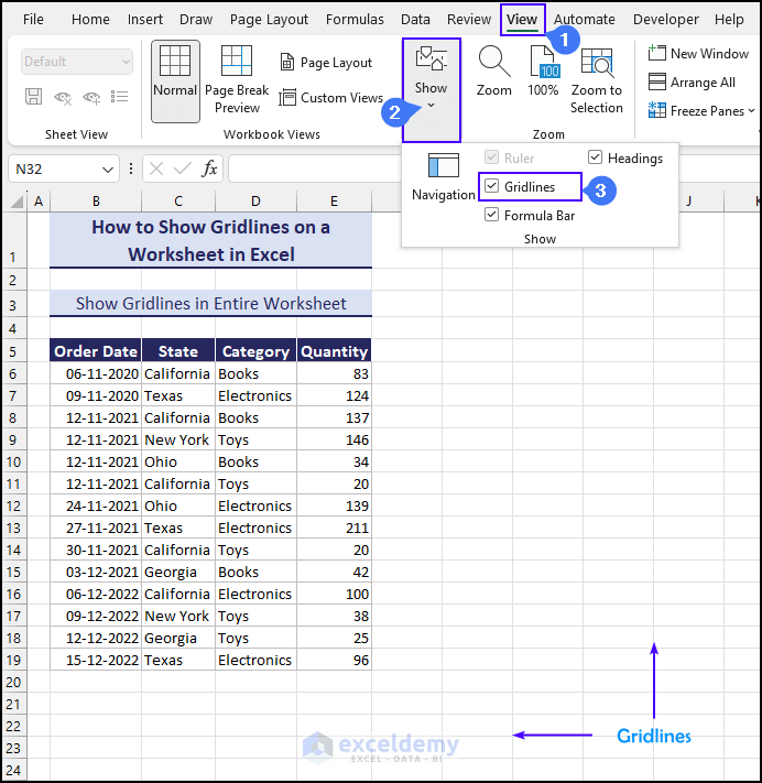
1. Using View Tab Commands
To show gridlines using the View tab commands follow the workaround below.
Go to View tab >> Show group of command >> Check the Gridlines option.
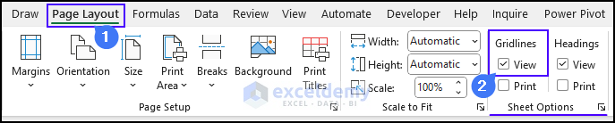
2. Using the Page Layout Tab Commands
As an alternative approach, visit the Page Layout tab and access the Gridlines column under the Sheet Options group of commands. Opt for the View option, and you will observe the gridlines appearing in the worksheet.
3. Using a Keyboard Shortcut
If you are having trouble spotting the gridline settings in Excel, well no worries. You can also use keyboard shortcuts.
As a matter of fact, just press ALT+W+V+G to turn on the gridlines if they are hidden. This shortcut acts like a switch. You can use it to turn on or turn off the gridlines in any worksheet.
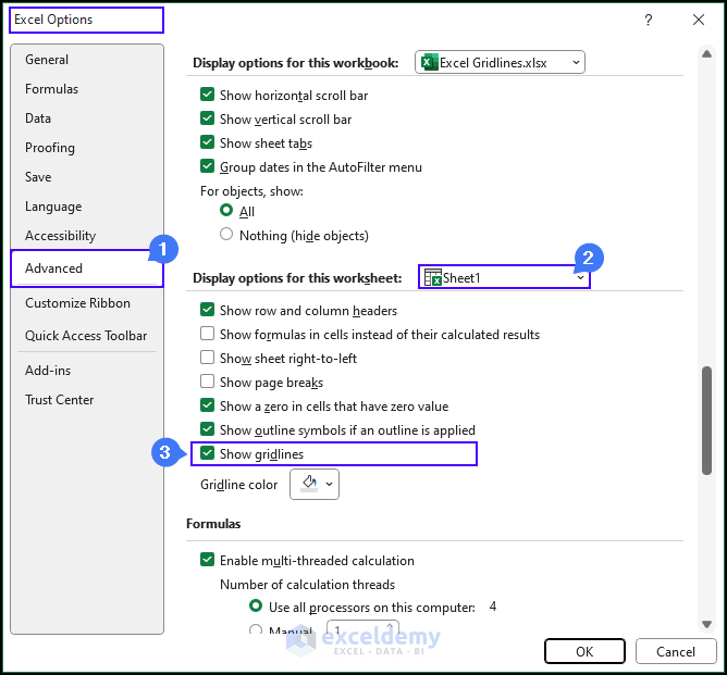
4. Using ‘Display options for this worksheet’ from Advanced Excel Options
Excel keeps the show/hide gridlines option in another place- Excel advanced options. To show gridlines using Excel advanced options-
- Press ALT+F+T. This will take you to the Excel options window.
- In the Excel Options window, choose Advanced from the left panel.
- Scroll down to Display options for this worksheet on the right panel.
- Next, select the worksheet and then check the Show gridlines box to show the gridlines in that sheet.
How to Turn Off Gridlines in Excel?
Users often hide gridlines for aesthetic purposes. For example, professional appearance, cleaner outlook, emphasizing the data, or for presentation or printing.
You can hide gridlines by turning them off. You can use the View command, Page Layout command, or the keyboard shortcut to turn off gridlines in Excel.
The quickest way to hide gridlines in Excel is to use the keyboard shortcut. Besides, it is applicable to all versions of Excel. You can simply press ALT+W+V+G to turn off the gridlines.
How to Hide Gridlines in Excel Without Turning Them Off?
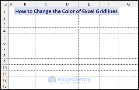
You can also hide gridlines for the entire sheet by changing the gridline color to white.
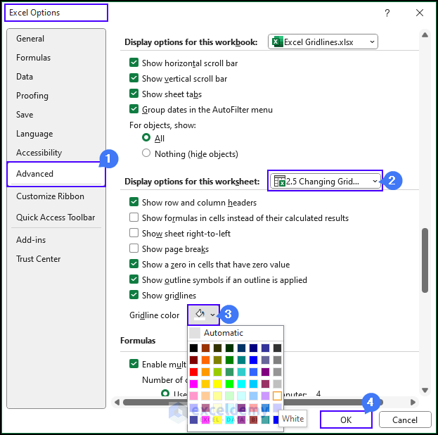
- Go to the File ⇒ Options.
- Navigate to the Advanced option. On the right, scroll down to locate “Display options for this worksheet.”
- Select the sheet where you want to apply the changes.
- Find the option to change the Gridline Color. Generally, it is light gray.
- Change the color to White and press OK to save the changes.
Return to the worksheet to witness the change. Even though the Gridlines option is checked in the View tab, it will not show any gridlines on the sheet.

Can We Show Gridlines for Specific Cells in the Worksheet?
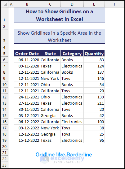
Unfortunately, there is no option to show gridlines only in a specific area in the worksheet. But you can mimic a gridline effect for specific cells by using Excel borders for that specific area of the worksheet and selecting a light gray color for the borders.
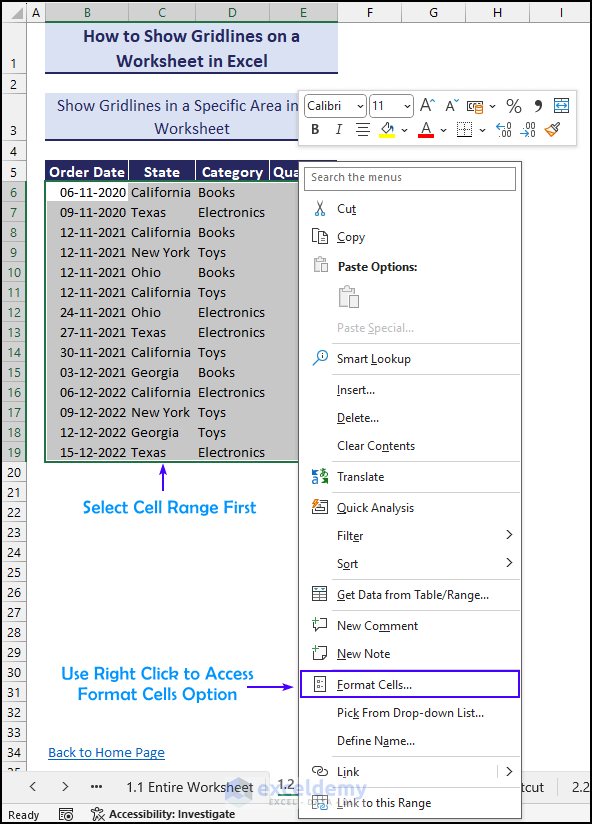
Let’s say, we want to apply gridlines (or mimic gridlines!) in cells B6:E19.

Follow the steps below to imitate gridlines for those specific cells.
- First, select the specific cell range B6:E19.
- Right-click on your mouse and select the Format Cells option from the context menu.
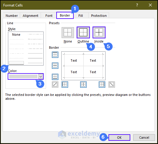
Now follow the steps in order or else you may face difficulties.
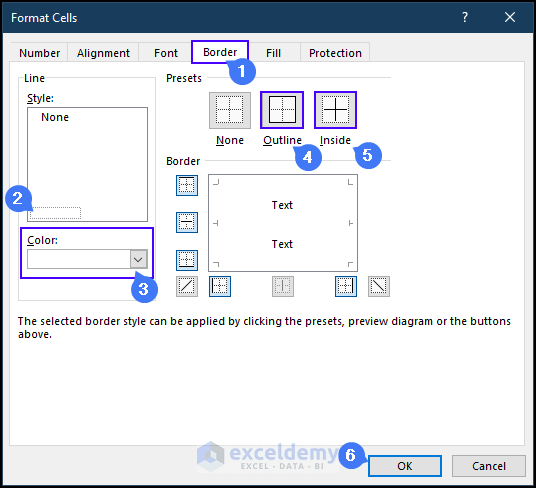
- Select Border Tab,
- Choose Style,
- We will choose White, Background 1, Darker 15% as the Border Color.
- Click the Outline and Inside options.
- Finally, Click OK to save the formatting.
Thus, You can make a specific cell range (B6:E19) look like default gridlines in Excel by applying border styles.
How to Hide Gridlines for Specific Cells in Excel?
You can hide gridlines for specific cells by using fill color or by changing the gridline color.
1. Using Fill Color
If you want to apply background fill to remove gridlines in a specific area, check the following steps.
- Select Cell/Region i.e. B6:E19
- Home Tab >> Font Group >> Fill Color drop-down menu.
- Select White as the Fill Color.
Finally, you can see that the Excel gridlines disappear when color is added.
2. Applying Borders and Changing Border Color
In this case, assume we have the following dataset and we will remove gridlines only in cells ranging from D6 to D12.

Steps:
- Select Border Tab,
- Choose Style,
- Choose White as the Border Color.
- Click the Outline and Inside options.
- Click OK to save the formatting.
In the end, you will have the following output. These specific cell ranges (D6:D12) are without any gridlines.
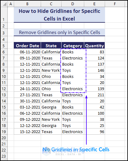
Thus you can hide gridlines on part of sheets in Excel.
How to Remove Gridlines from Multiple Worksheets
The easiest way to remove gridlines from multiple worksheets is to press and hold CTRL while selecting the desired sheets. Once selected, you can do any of the following:
1. Go to the View tab and uncheck the Gridlines option.
2. Navigate through the Page Layout tab and uncheck the View option from the Gridlines column.
Any of these actions will remove gridlines across all the chosen worksheets straightaway.
Read More: How to Remove Grid from Excel
How to Change the Color of Excel Gridlines
You can make gridlines darker by changing their color. Check the following steps.
- File tab >> Options menu.
- After that from the Excel Options window, go to the Advanced option.
- Find “Display options for this worksheet” and select the sheet you want to modify explicitly.
- Then, find the Gridline Color Option.
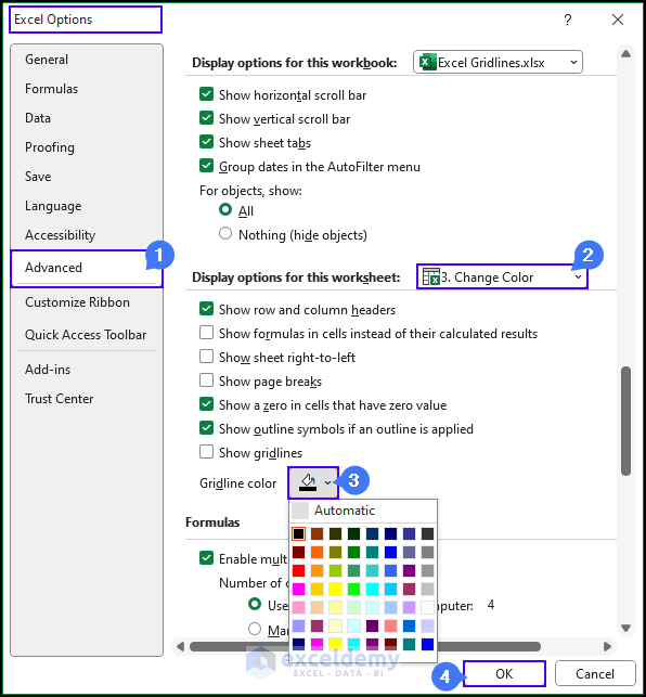
In this case, we are going to change it to black to make the gridline thicker and press OK to save the change.
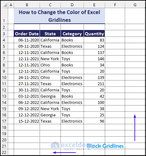
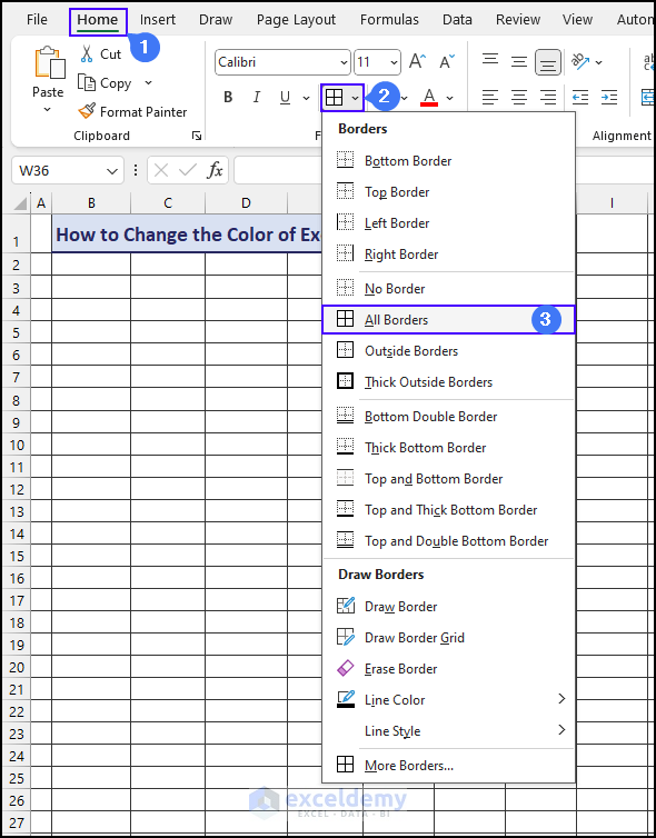
When you change the color of gridlines, you may notice that the gridlines become dotted like this-
If you find this issue problematic, then you can apply all borders after changing the color. Using the following steps you can easily.
Home Tab >> Borders drop-down menu >> All Borders.
How to Show Gridlines After Using Fill Color in Excel
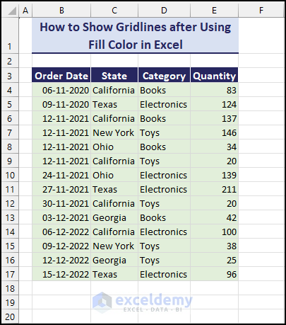
As soon as we apply the Fill Color feature to color the cells, the gridlines technically disappear, which may not always be desired. In the following dataset, we’ll demonstrate the steps to show gridlines after using the fill color.
- First select the cell range for this example, cell range B4:E17.
- Go to Home tab >> Font Group >> Borders drop-down menu >> More Borders option.
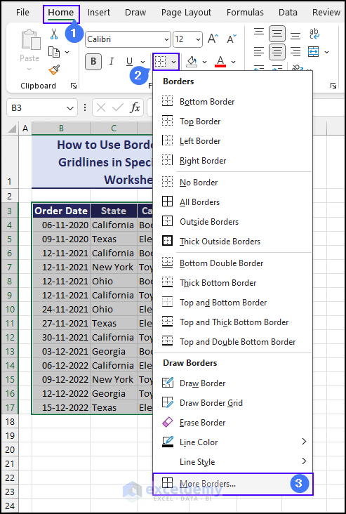
- Now select the Border Tab,
- Choose Border Style,
- Afterward, we will choose White, Background 1, Darker 15% as the Border Color.
- Then, Click the Outline and Inside options.
- Finally, Click OK to save the formatting.

It will restore the gridlines in the cells that were previously filled with color.
Read More: Excel Fix: Gridlines Disappear When Color Added
How to Print Gridlines on a Worksheet in Excel
By default, Excel does not include gridlines when printing. To print gridlines, follow these steps:
- Navigate to the Page Layout tab.
- In the Sheet Options group, locate the Gridlines column.
- To print gridlines, check the Print option. This will instruct Excel to include gridlines on the printed paper surely.

An alternative way is printing gridlines directly from the Page Setup menu. Check the following steps:
- File Menu >> Print Option >> Page Setup
- From the Page Setup Window, go to the Sheet tab.
- Check the Gridlines Option under the Print section.
- Click OK to save the change.

This concludes our tutorial on Excel gridlines. Here you have learned what Excel gridlines are and how you can show or hide them in Excel. You have also learned how you can mimic gridlines using Fill Color or Borders commands. In case you only need to show or hide gridlines for specific cells, you can do that by imitating gridlines as shown in this tutorial. In the end, we have also shown how to change gridline color, how to show them even after using fill color, and how you print gridlines on your worksheet. Please let us know your feedback in the comment box.
Gridlines in Excel: Knowledge Hub
- Why Do Gridlines Disappear in Excel?
- Add Gridlines in Excel
- Show Gridlines in Excel
- Edit Gridlines in Excel
<< Go Back to Gridlines | Learn Excel

