There are several ways to highlight a cell in Excel, among them we will demonstrate to you 5 easy and effective methods.
How to Highlight a Cell in Excel: 5 Methods
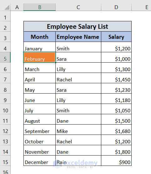
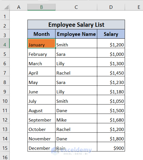
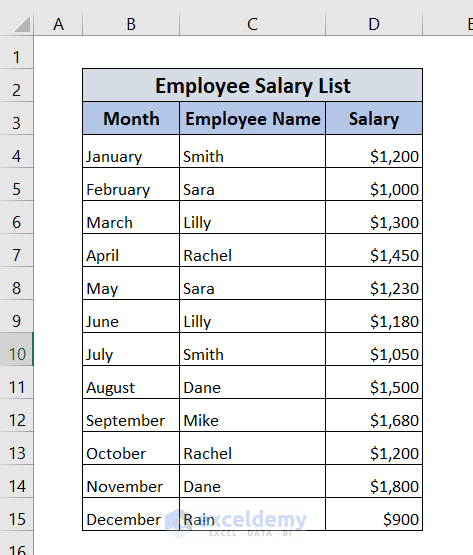
The following Employee Salary List table shows the Month, Employee Name, and Salary column. In this table, we want to highlight a cell using 6 different methods. Here, we used Excel 365. You can use any available Excel version.

Method-1: Cell Styles to Highlight Cells in Excel
From the following Employee Salary List table’s Month column, we want to highlight the month of February.

To begin with, we will select the cell we want to highlight. Here, we want to highlight February, therefore, we select cell B5.
➤ After that, we will go to the Home tab in the Ribbon. Then, we have to select Cell Styles.

Now, we will see a menu with a variety of cell color options pop up. We will hover our mouse cursor over each color, and we will see a live preview of the cell color change in the Excel file.

Here, we can see that when we hover our mouse on Accent2 to Highlight our cell, our cell F4 becomes highlighted with that color.
➤ Now, we will click on Accent2.
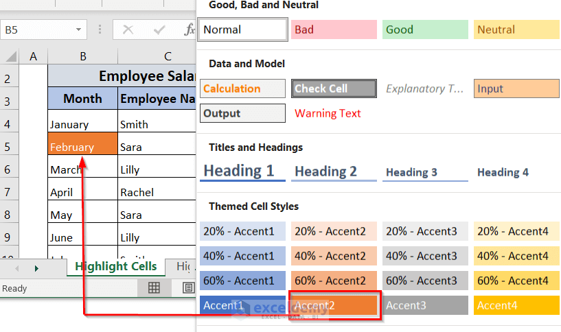
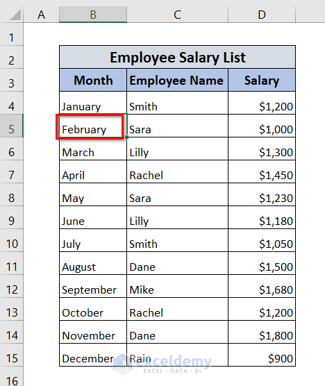
Finally, we can see that the month of February is highlighted.
Method-2: Highlight Text in a Cell
Highlighting cell often means highlighting text. In this method, we want to highlight the text in cell B5.
➤ Now, we will double-click on cell F4.
➤ After that, right-click on cell F4.
Now, we can see that a context menu is appearing.
➤ From that menu, we have to click on the down arrow from the option marked as 2 in the following picture.

After that, we will see a variety of colors appear, and we can select any of them.

When we hover over these colors with our mouse cursor, we can see the preview in our selected cell. Here, we can see that when we hover over the red color with our mouse cursor, the text in our cell F4 becomes red.
➤ Now, we will click on this red color.

Finally, we can see the text in cell F4 is highlighted with red color.

Method-3: Create a Microsoft Excel Highlight Style
In this method, whenever we do not like the default cell style options, we can create our own highlight style.
To do so, first, we have to open our Excel document.
➤ After that, we will go to the Home tab in the Ribbon. Then, we will select Cell Styles.

➤ Now, we will select New Cell Style.

A Style window will appear, and we have to give a Style name.
Here, we give the name Highlight 1.
➤ After that, click on Format.

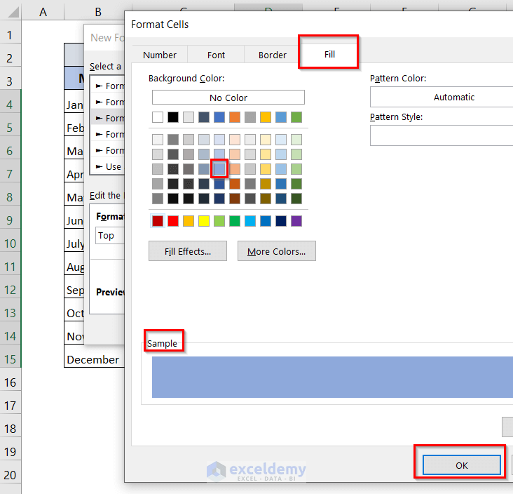
➤ After that, a Format Cells window will appear.
We have to select Fill
➤ Then, select a Color.
We can see the preview of the color in the Sample. Now, we will click on OK.

➤ Now, we will click OK in the Style window.

Now, we can see our created cell style Highlight 1 in the Cell Styles option.
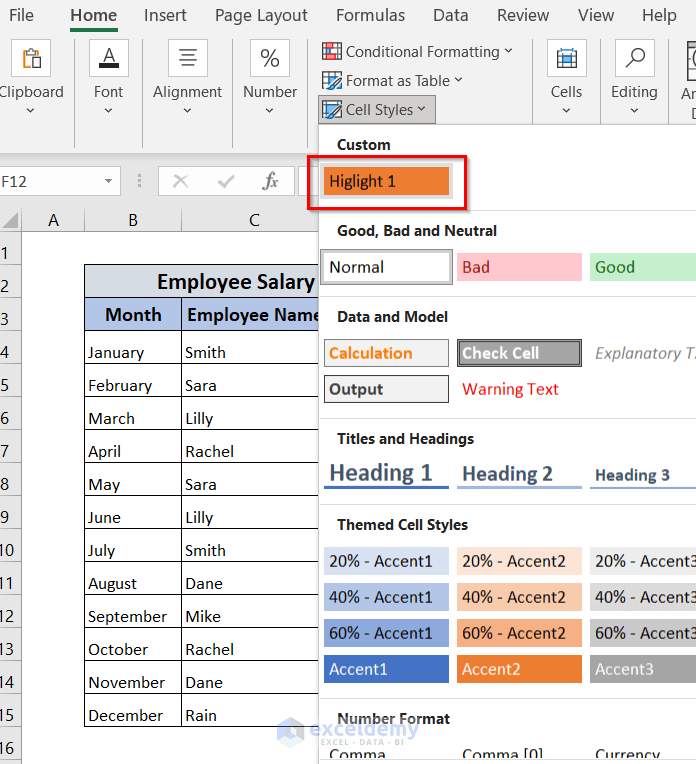
➤ Now, if we select cell B4, and hover our mouse on Highlight 1, we can see that cell B4 is highlighted with the color as Highlight 1.
➤ Now, we will select Highlight 1.

Finally, we can see that our cell B4 is highlighted with our created highlight style. We can apply this style to any of the cells according to our choices.
Method-4: Use Conditional Formatting to Highlight a Cell
In this method, we will use Conditional Formatting to Highlight cells in 4 different cases.
Case-1: Highlight Cells Above a Specific Number
In this case, we want to Highlight Salary that is above $1200.
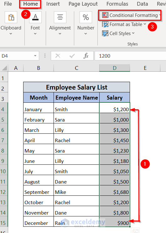
First of all, we have to select the entire data range from the Salary column.
➤ Then, go to the Home tab in the Ribbon, and then, select Conditional Formatting.
After that, select Highlight Cells Rules.
➤ Then, select Greater Than.

Now, a Greater Than window will come.
➤ We will type 1200 in the box Format cells that are GREATER THAN.
After that, we will select a Custom Format according to our choices.
➤ Here, we select Green Fill with Dark Green Text.

➤ Now, click on OK.

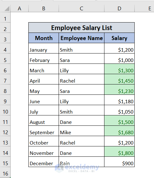
Finally, we can see the salary above $1200 is highlighted.
Case-2: Highlight Top 5 Entries
In this case, we want to highlight the top 5 salaries in the Salary Column using Conditional Formatting.
To begin with, we will select the entire data range of the Salary column.
➤ Then, we will go to the Home tab in the Ribbon. We will select Conditional Formatting.

➤ Now, we will select Top/Bottom Rules, and then, select More Rules.

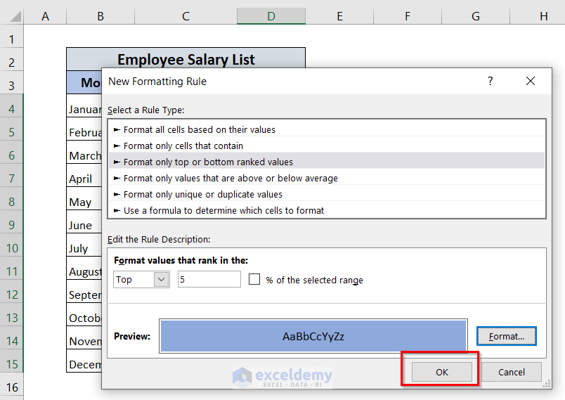
A New Formatting Rule window will come in front of you.
➤ We will type 5 in the box marked as 1 in the following picture.
➤ Then, we will click on Format.

A Format Cells window will appear.
➤ Now, we will select the Fill option.
We will select a color according to our choices. Here, we select the blue color.
➤ We can see the selected color in the Sample box. Now, click on OK.
➤ Now, click on OK in the New Formatting Rule window.
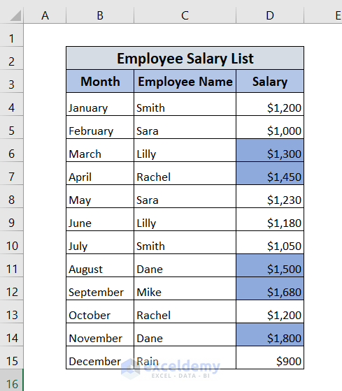
Finally, we can see the top 5 salaries highlighted in blue color in the Salary column.
Case-3: Show Data Bars Instead of Color Shading
In this case, instead of Color Shading, we want to Highlight Salary with Data Bars using Conditional Formatting.
First of all, we will select the entire data range of the Salary column.
➤ Then, we will go to the Home tab in the Ribbon. We will select Conditional Formatting.

➤ After that, we will select Data Bars.
➤ Then, select More Rules.

A New Formatting Rule window will pop up.
➤ We will mark on the box Show Bar Only.
➤ We will choose a Color. Here, we select the yellow color.
We can see the preview of the color in the Preview box.
➤ Then, click on OK.

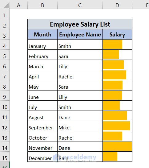
Finally, we can see the Highlighted Data Bars in the Salary column with Yellow Color.
Case-4: Highlight a Row in Excel
In this case, we want to highlight an entire row where the salary is greater than $1000 by using Conditional Formatting.
To begin with, we will select the entire dataset from cells B4 to D14 from the Employee Salary List table.
➤ After that, we will go to the Home tab in the Ribbon. We will click on Conditional Formatting.
➤ Then, click on New Rules.

A New Formatting Rule window will come in front of you.
➤ We will select Use a formula to determine which cells to format options.
In the Format values where this formula is true box, we will type =$D4>1000.
➤ After that, we will select Format.

Now, a Format Cells window will pop up.
➤ We will select the Fill option
We have to choose a Color, here, we choose Green. We can see the color in the Sample box.
➤ Then, we will click on OK.

➤ After that, in the New Formatting Rule window, we can see the Preview of the color.
➤ We will click on OK.

Finally, we can see that the rows having salaries greater than $1000 are highlighted with green color.

There are many scenarios like highlighting the active row and column, and so on that can be matched using the Conditional Formatting feature.
Read More: Highlight Blank Cells with Conditional Formatting
Method-5: Find and Highlight Cell in Excel
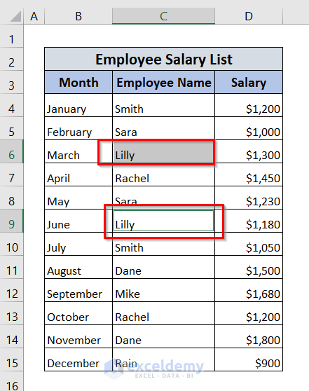
In this method, we want to find the Employee Name Lilly, and we want to Highlight it with red color.
First, we will go to the Home tab in the Ribbon.
➤ After that, Select the Editing option.
➤ Then, select the Find & Select option. And then, select the Find option.

Now, a Find and Replace window will appear.
➤ We will type Lilly in the Find What box.
➤ And we will click on Find All.

Now, we can see at the button of the Find and Replace window our search values.

➤ Now, we will select one line in the found cells and press CTRL + A on the keyboard to select all cells.
➤ Then, click Close.

Now, all cells containing Lilly are selected (C6 and C9).
➤ Now, to highlight them, in the Ribbon, we have to go to the Home tab.
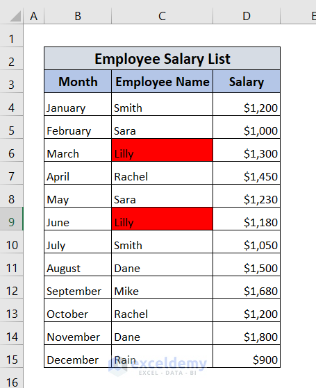
➤ Then, we will click on Fill Color, and we will select Red Color.

Finally, we can see that all cells that contain the name Lilly are highlighted in red.
Read More: Highlight Selected Cells
Download Workbook
Conclusion
Here, we tried to show you some easy and effective methods that will help you to Highlight a Cell in Excel. We hope you will find this article helpful. If you have any queries or suggestions, please feel free to contact us in the comment section.
How to Highlight a Cell in Excel: Knowledge Hub
- Highlight Cell If Value Is Less Than Another Cell
- Highlight Cells in Excel but Not Print
- [Fixed!] Cells Are Not Highlighting in Excel Formula
- Highlight Cells in Excel Based on Value
- Click One Cell and Highlight Another
- Highlight Cells Based on Text
- Highlight Cells That Contain Text from a List
- Highlight Cell Using the If Statement
<< Go Back to Highlight in Excel | Learn Excel

