In this tutorial, you will learn how to format addresses in Excel. You will find four different techniques by which you will be able to format your address in Excel. In addition to that, you will learn how to create a mailing address from a given address.
We have used Microsoft 365 to prepare this article. But you can use these methods in Excel versions from Excel 2003 onwards.
Generally, we use address formatting in Excel to present data in a consistent manner. It helps us to split addresses into different components or combine components into one. Formatting addresses makes the comparison or sorting of addresses easier by ensuring consistency. Above all, it helps reduce data entry work and improves the accuracy of the data. The easiest of all these methods is using the Flash Fill feature. If you are comfortable with using functions then you have various options in your hand to format address. A lot of functions are available in Excel to help you format your address.
Download Practice Workbook
Overview of Standard Address Format
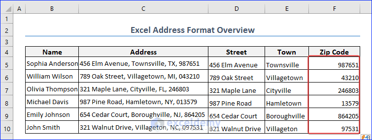
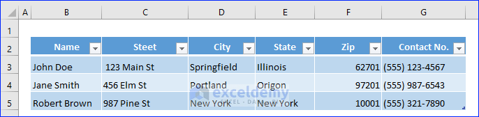
While formatting addresses in Excel, we need to follow some standard rules. For example, house and building numbers should be in the first line. City and state numbers will appear in the next part of the address. In the standard format, the zip code appears in the last part of the addresses. You should pay special attention while working with the Zip code. Some of the zip codes start with “0”. If you don’t format the column as Zip Code, it will remove the leading zero.
Click to see full image
In the image above, you will find that Excel has automatically removed the leading zero. So, we will format the Zip Code column to solve the issue.
- Select the column and press Ctrl+1
- In the Format Cells dialog box, choose options like the image below.
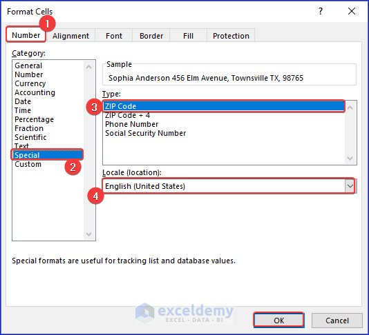
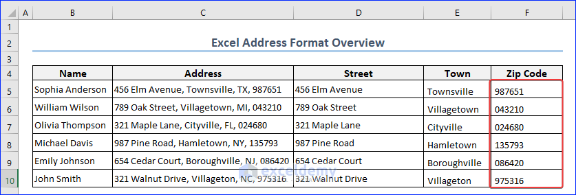
After that, you will find that Excel is not removing the leading zero anymore.
Click to see full image
Read More: Organize Addresses in Excel
How to Format Address in Excel
1. Use Excel Features
1.1 Applying Text to Columns Command
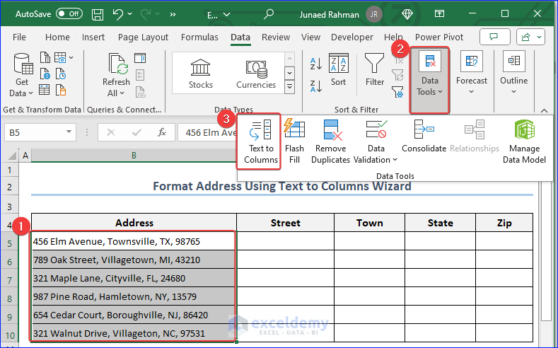
To format address using the Text to Columns wizard
- Select the data in Column B (B5:B10). Click on the Data tab>>Data Tools>>Text to Columns wizard.
Click to see full image
After selecting the wizard, you will find 3 dialog boxes that will appear one by one. Choose the following options in those dialog boxes.
- Delimited in the first dialog box.
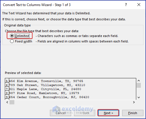
- If you look at the address in our dataset, you will find that different parts are separated by commas. So, choose Comma in the delimiters group.

- In the last one, you needn’t do anything. Just click on Finish.
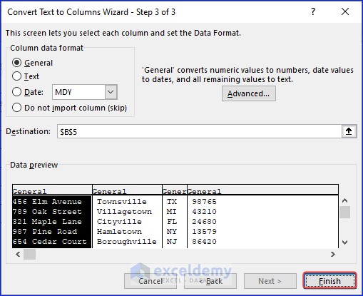
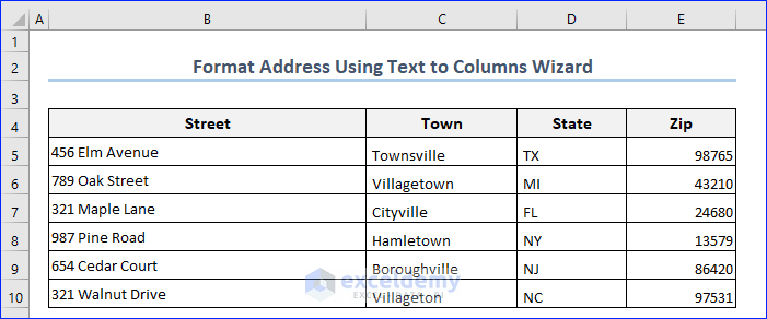
The output is similar to the following image.
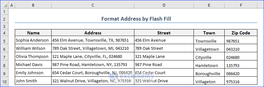
1.2 Use of Flash Fill Feature
- First, select the cell that contains the address. Then, copy up to the first comma (the street part of the address) and paste it into the D5
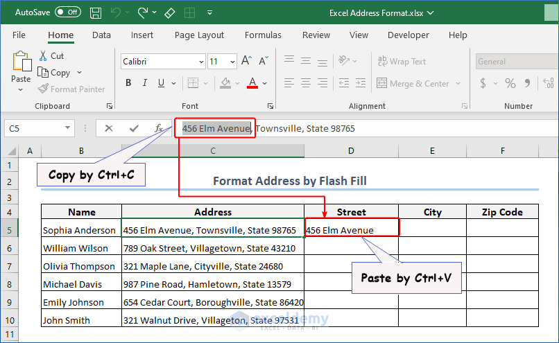
Click to see the full view of image
- After that, double-click on Fill Handle to copy the formula up to cell D10.
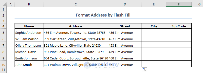
Click to see the full view of image
Excel fills the blank cells with the Fill Series option. However, we will change this to the Flash Fill option in order to get the desired output.
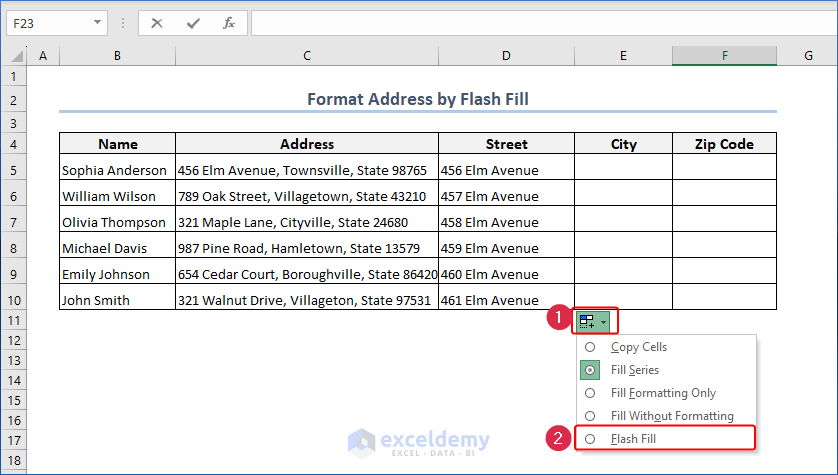
Click to see the full view of image
So the output image will be as follows.
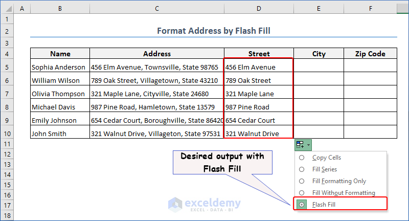
Click to see the full view of image
Click to see full image
The final output will be similar to the following image.
When to Use Excel Features or Non-Formula Methods to Format Address?
Using Excel features is quick and easy. They are especially useful in the following cases.
- If you import data from a website or reporting system.
- When you are not that much expert at formulas.
- Scenarios where you don’t want to change the main address.
On the other hand, if you use features to format addresses, data may not update automatically.
Read More: Format Addresses in Excel
2. Use Excel Formulas to Format Address
2.1 Using FIND, LEFT, MID, and RIGHT Functions
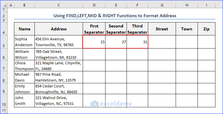
Step 1: Finding Separator Positions
In this method, we will use FIND, LEFT, MID, and RIGHT functions. We need to define the starting and end positions in the arguments of these functions. For example, to get the street portion of the address, we need to mention the position of the first comma in the argument of the LEFT function. In the same way, the position of the second and third comma is necessary to get the Town name of the address.
1st Separator: Apply the following formula in the cell. We will apply this in cell D5.
=FIND(",",C5)
FIND(“,”,C5): Here, the searching criteria is a comma and the text where we will perform searching is cell C5. We will get the position of the first comma.

Click to see full image
2nd Separator: The FIND function returns the position of the first appearance of any character. To get the second one, in this case, the search will have to start from the next position of the first comma, which is D5+1.
=FIND(",",C5,D5+1)
3rd Separator: Modify the formula to find the 3rd separator. Replace the D5+1 argument with E5+1. You will get the position of 3rd separator.
=FIND(",",C5,E5+1)So, you’ll get 1st, 2nd and 3rd seperators.
Click to see full image
Step 2: Insert Street Address Formula
We will separate street addresses using the LEFT function. Apply the following formula to cell G5 and hit ENTER. Use AutoFill to fill up the remaining cells.
=LEFT(C5, D5-1) The LEFT function extracts a part of a text according to the position we define. In this case, we defined the position before the comma. So, the formula will extract all the things that it finds before that comma.
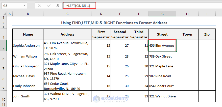
Click to see full image
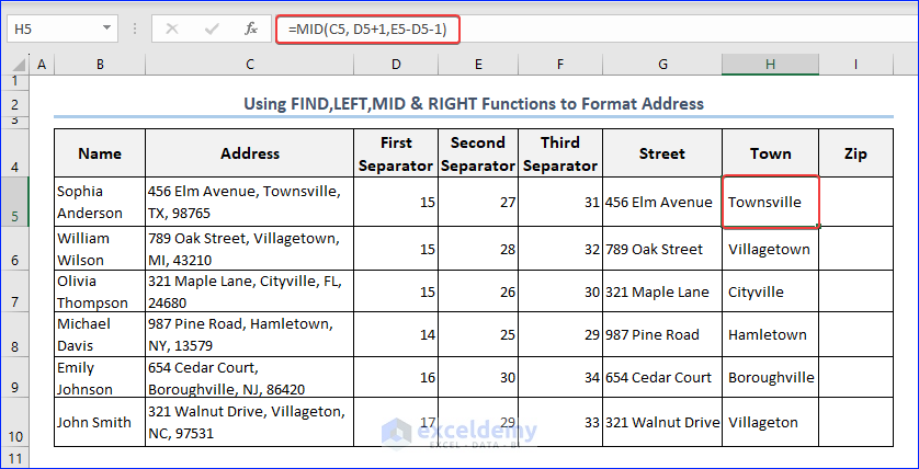
Step 3: Separating Town Name
We will use the MID function to find out the Town address from a given address. Just put the following formula in the cell and get the result.
=MID(C5, D5+1,E5-D5-1)🔎 Formula Breakdown
- C5: The first argument of the MID It is the text from which the function will extract some characters.
- D5+1: Defines where the MID function starts to extract characters.
- E5-D5-1: Indicates the end of extraction of MID
The output will look like the following one.
Click to see full image
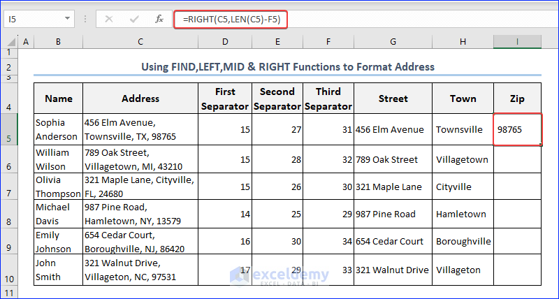
Step 4: Separating Zip Code
Write the formula in I5 cell to separate Zip.
=RIGHT(C5,LEN(C5)-F5)🔎 Formula Breakdown
- LEN(C5): Finds the length of the text C5.
- LEN(C5)-F5: Subtracts the position of the 3rd separator from the length of C5 to get how many characters the RIGHT function would extract.
- RIGHT(C5,LEN(C5)-F5): Extracts all the characters that are present after the 3rd comma.
Click to see full image
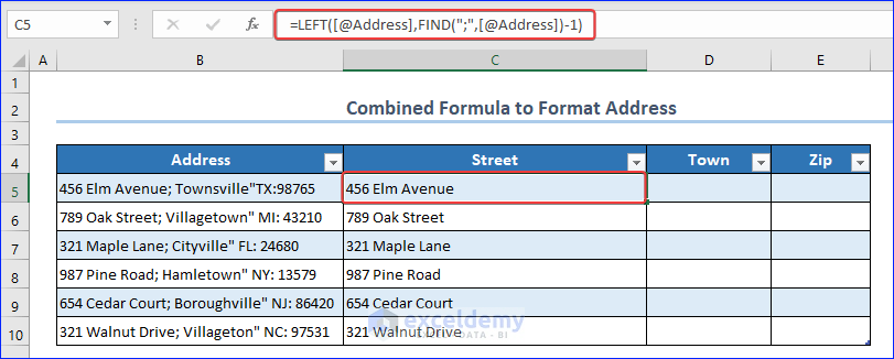
2.2 Using a Combined Formula When Delimiters Are Not Same
- First, convert the range into a table by pressing Ctrl+T
- Apply the following formula in the cell C5.
=LEFT([@Address],FIND(";",[@Address])-1)You will get the street address in Column C.
Click to see full image
🔎 Formula Breakdown
- FIND(“;”,[@Address]): Returns an array that contains the position of the delimiter “;” in the address.
- LEFT([@Address],FIND(“;”,[@Address])-1): Extracts the values that appear before the delimiter “;”.
Getting Other Values:
In order to get the town names, use the following formula in your worksheet. We will apply this in the cell D5.
=MID([@Address], FIND(";", [@Address]) + 2, FIND("""", [@Address], FIND(";", [@Address]) + 2) - (FIND(";", [@Address]) + 2))To get the Zip code, we will use the following formula in the cell E5.
=MID([@Address], FIND(":", [@Address]) + 1, 6)The final output will be similar to the following image.
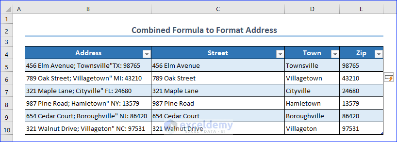
Click to see full image
2.3 Using TEXTBEFORE and TEXTAFTER Functions
- Firstly, apply the following formula at cell D5 and hit ENTER, use the AutoFill feature to fill up the remaining cells.
=TEXTBEFORE(C5,",")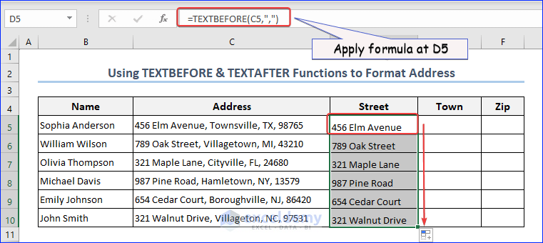
Click to see full image
- It’s now the turn of Town. We will apply the following formula at E5 and repeat the same procedure of finding Street.
=TEXTBEFORE(TEXTAFTER(C5,",",1),",",1)Here, TEXTAFTER(C5,”,”,1) finds the text after the first comma in C5, which is Townsville, TX, 98765. Then, the TEXTBEFORE function takes Townsville, TX, 98765 as its first argument and finds the content before the first comma in it; which is Townsville.
The output looks like the following image.
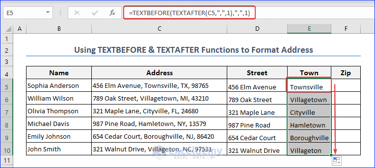
Click to see full image
Finally, we will find the Zip code in the Zip column. Apply the formula at F5 and use AutoFill like before.
=TEXTAFTER(C5,",",3)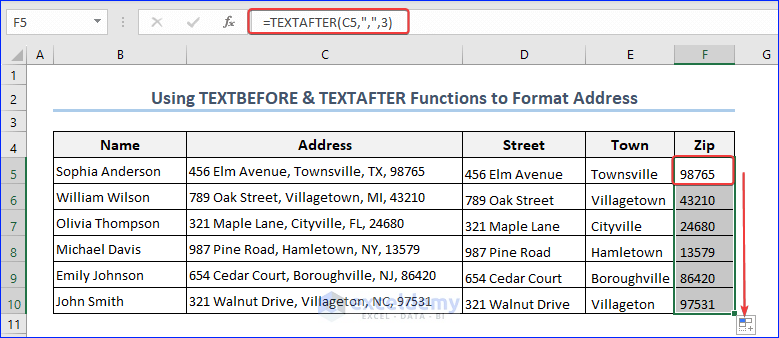
Click to see full image
2.4 Using TEXTSPLIT and CHOOSECOLS Functions
- Write down the formula in the first cell under the Street
=CHOOSECOLS(TEXTSPLIT(C5,","),1)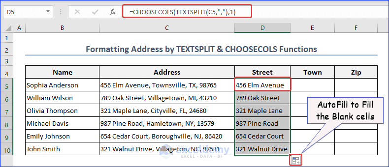
Click to see full image
In order to find the Town, we will modify the formula and put 2 in place of 1 in the argument of the CHOOSECOLS function. As a result, now we will get the second value in the array, which is “Townsville”.
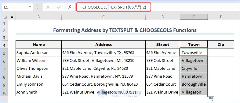
Click to see full image
Finally, we will find the Zip code by changing the last argument of the CHOOSECOLS function to 4. The output will be similar to the following image.
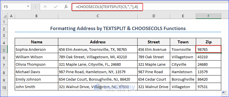
Click to see full image
When to Use Formula Method to Format Address in Excel
Formatting addresses using formulas is beneficial when we need dynamic and automated data manipulation. These methods are:
- Flexible &
- Can handle complex transformations.
Some negative sides of using formulas are:
- Requires sound knowledge of formulas and
- Slower for large datasets
Read More: Make an Address Book
3. Using Power Query to Format a One-Column Address List
We have a column that contains the names and addresses of some employees in a company. We will convert it to readable table format.
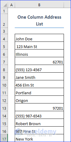
- Convert the list into a table by pressing Ctrl+T.
- Open the table in Power Query
- In the Power Query editor, add an Index Column from the Add column option.
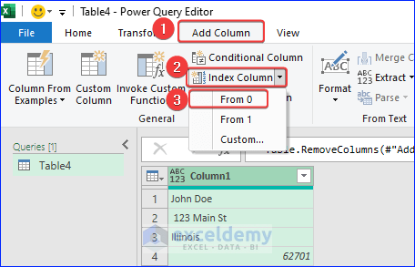
The output of adding the Index Column:

In the list, you will find that each employer’s address expands to consecutive 6 rows (Including name). If we assign numbers in such a way that will start from 0 for the first data of each employee and then go to the last data entry of that employee and again start from 0 for another employee, it will be a good technique.
- Select Standard >>Modulo option.

- A dialog box named Modulo will appear where we will input value “6” since each employee data expands to consecutive 6 rows.
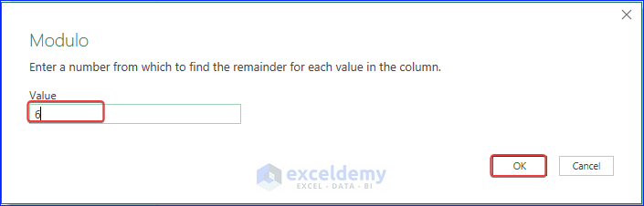
The output of adding a Modulo column looks like the following image.

- Now, we will transform address data into columns. Select the options like the following image in your dataset.
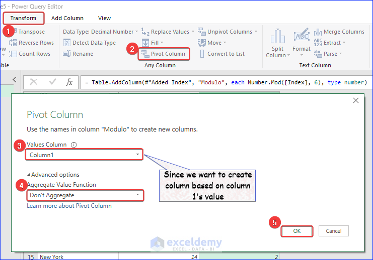
You will get an output like the following image.
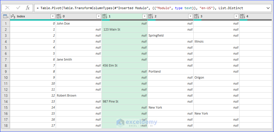
Click to see full image
- Holding down the Shift key, select Column 1 to Column 5.
- From the Transform tab, select Fill >> Up.
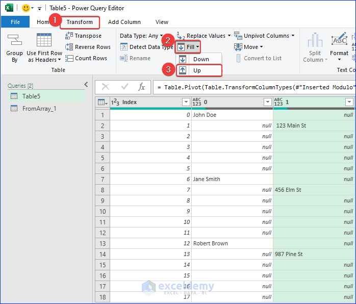
The output of this step is similar to the following image.
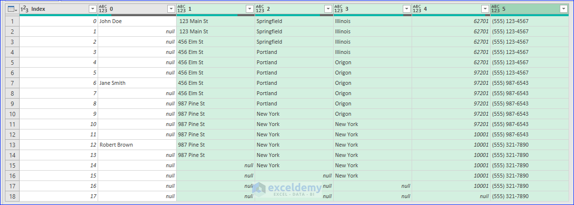
Click to see full image
- After that, we will click on the drop-down arrow of Column 0 and deselect the option “Null”.
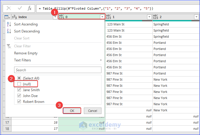
- Delete the Index Give proper names to the columns like the following image

Click to see full image
Finally, click on Close & Load to see the results in your worksheet.
Read More: Formula to Create Email Address
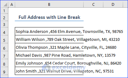
How to Format Full Address in One Cell with Line Break in Excel
In order to format the full address in one line, we will use the line break instead of the Wrap Text option. We have a dataset in Excel like the following image. We want to increase the readability of the addresses.
- First, we will try the Wrap Text The output looks like the following image. (You will have to adjust the row height to make the address readable. We set it to “30”)
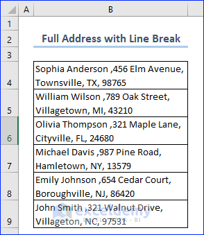
Looking at the image above, you will decide that the address is not correctly formatted since you cannot differentiate different parts of it. To solve this, we will apply line break.
Process Description
- Click on cell B4 and place your cursor right after the first comma after the name “Sophia Anderson”
- Delete the comma by pressing Backspace. Press Alt+Enter together to insert new line.
- In the same way, place your cursor after the 3rd comma, delete it and insert new line.
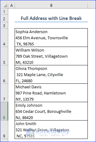
- Repeat the whole process for all the cells and finally change the Row Height to 45.
The output is similar to the following image.
Read More: Excel Formula to Create Email Address with First Initial and Last Name
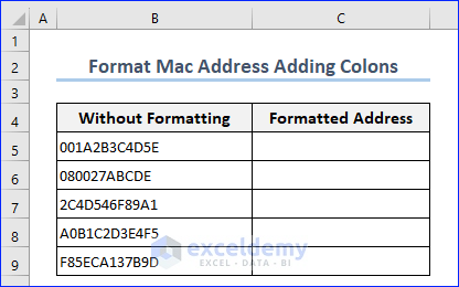
How to Format Mac Addresses in Cells by Adding Colon Symbol in Excel
We have the following dataset in Excel. We will format them as Mac addresses.
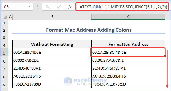
- Apply the following formula in C5 and hit ENTER to get the result.
=TEXTJOIN(":",1,MID(B5,SEQUENCE(6,1,1,2),2))- Use the Fill Handle feature to get addresses in the other cells as well.
The output is similar to the following image.
🔎 Formula Breakdown
- SEQUENCE(6,1,1,2) = {1,3,5,7,9}: Generates an array of 6 numbers starting from 1 and an increment of 2.
- MID(B5,SEQUENCE(6,1,1,2),2) = {00, 1A, 2B, 3C, 4D, 5E}: It also generates an array that extracts consecutive 2 characters from B5 according to the array generated by the SEQUENCE function.
- TEXTJOIN(“:”,1,MID(B5,SEQUENCE(6,1,1,2),2)) = 00:1A:2B:3C:4D:5E: Joins the array elements generated by the MID function with a colon between them.
How to Find Mailing Address from Name and Address?
In Excel, we can combine the name and address of a customer to find out the mailing address. We will use the SUBSTITUTE function to do that. Our dataset looks like the following image.

- At this point, we will apply the following formula in cell D5, hit Enter, and apply Wrap Text to the cell.
=SUBSTITUTE(B5&CHAR(10)&C5,", ",CHAR(10),1)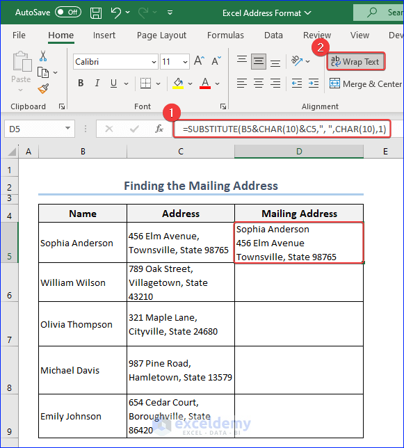
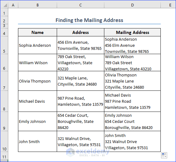
- After dragging the Fill Handle, the output will be as follows.
🔎 Formula Breakdown
- “,”&CHAR(10) : Char(10) is the character that adds a new line in Excel. So, this part adds a comma and then adds a new line to the cell.
- B5&CHAR(10)&C5 : Concatenates the content of B5 with C5 and adds the C5 in a new line.
- SUBSTITUTE(B5&CHAR(10)&C5,”, “,CHAR(10),1) : Replaces the first comma in the combined text of B5, CHAR(10), and C5 with CHAR(10). In other words, it replaces the first comma with a new line character.
Read More: Format a Column for Email Addresses
Things to Remember
- First of all, identify the specific components of the address you need to work with, such as street, city, postal code, country, or any other relevant information.
- Use consistent formatting across all address entries in your dataset. It will help you analyze the address.
- Since Excel automatically removes leading zero, pay attention to leading zeros in postal codes or other numerical components of an address.
Frequently Asked Questions
1. What are some common challenges in address formatting?
Answer: Some of the most common challenges in address formatting are: inconsistent formats, missing components, leading zeros, and data entry errors.
2. Can I combine separate address components into a single cell in Excel?
Answer: You can use some built-in functions of Excel to combine separate addresses into a single cell. You may use CONCATENATE or TEXTJOIN functions. Also, you may use the Ampersand operator or custom formula to do that.
3. Can I import or export address data with specific formatting requirements in Excel?
Answer: You can use CSV, .txt, or VBA macros to import and export data with specific formatting requirements.
Conclusion
Hey! You have reached the end of the article on Excel address format. The easiest way to format address is to use the Flash Fill feature. Also, you can use the FIND, MID, or LEFT functions to format addresses. Moreover, if you have Microsoft 365 subscription, you may use the TEXTBEFORE and TEXTAFTER functions. Hopefully, you enjoyed all the items covered in the article and you will apply these methods in your worksheet to format your address. If you find this article helpful, please share it with your friends. Moreover, do let us know if you have any further queries. Finally, please visit our site for more exciting articles on Excel.
Excel Address Format: Knowledge Hub
<< Go Back to Text Formatting | Learn Excel

