You may be accustomed to using the Sort & Filter option for sorting your data but there is a way to do this by using the Excel VBA SORT function also. By using this function the sorting task will be easier and faster than the conventional sorting method. So, let’s dive into the main article to know more about the Excel VBA SORT function.
Download Workbook
8 Ways to Use Excel VBA SORT Function
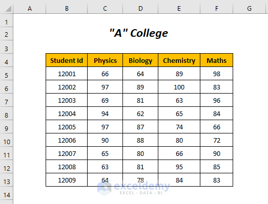
Here, we have used the following two data tables; one contains the sales records of a company,

and the other one has the records of marks of different students of a college. By using these tables we will demonstrate the ways of using the Excel VBA SORT function.
We have used Microsoft Excel 365 version here, you can use any other versions according to your convenience.
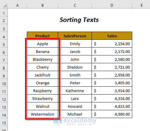
Method-1: VBA SORT to Arrange a Group of Texts
Here, we will sort our data based on the texts of the Product column.

Step-01:
➤ Go to Developer Tab >> Visual Basic Option.
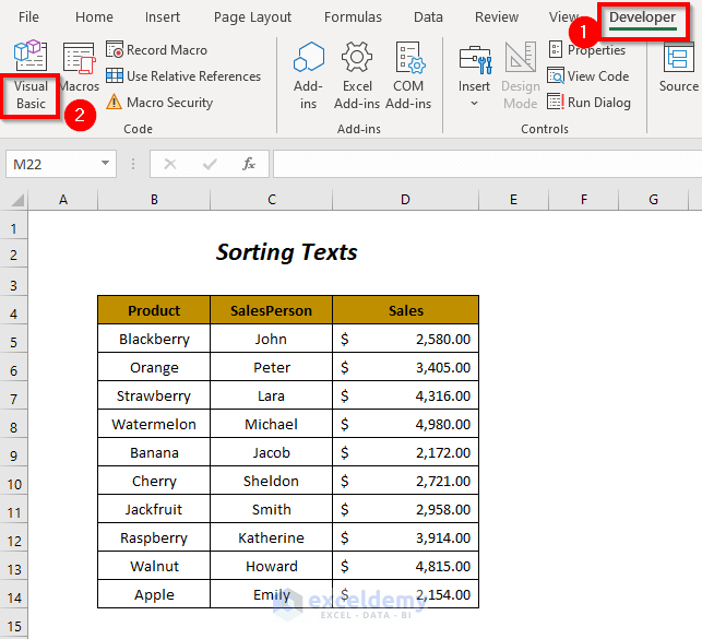
Then, the Visual Basic Editor will open up.
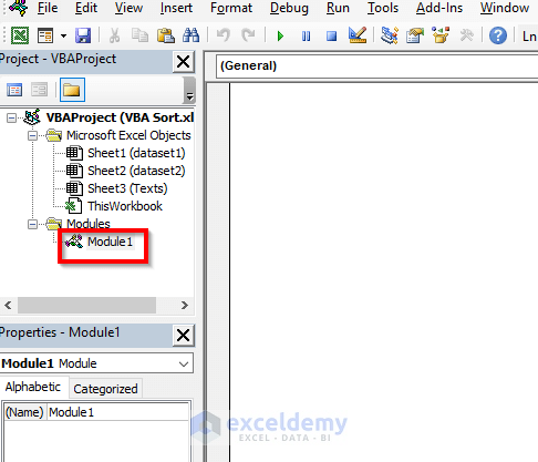
➤ Go to Insert Tab >> Module Option.

After that, a Module will be created.
Step-02:
➤ Write the following code
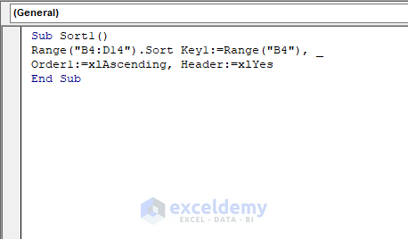
Sub Sort1()

Range("B4:D14").Sort Key1:=Range("B4"), _
Order1:=xlAscending, Header:=xlYes

End Sub
We have declared the range “B4:D14” to sort all of the values of this range and Key1 is the data range on the basis of which we are sorting our values, here it is Range(“B4”) because we want to sort on the basis of Column B, then Order1:=xlAscending indicates that the sorting order of this column will be from low value to high value, and finally Header:=xlYes will determine the first row of our range as a header.
➤ Press F5.
Then, you will get the sorted data on the basis of the Product column where the sorting appears in Ascending order (Excel considers A as the lowest value and Z as the highest value and so they are organized from low to high value).
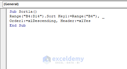
For arranging the texts from a high value (Z) to a low value (A) you can use the following code.
Sub Sort1a()

Range("B4:D14").Sort Key1:=Range("B4"), _
Order1:=xlDescending, Header:=xlYes

End Sub
This code is quite similar to the previous one except for Order1:=xlDescending, which means the order of the sorting process will be from a smaller value to a larger value.
➤ Press F5.
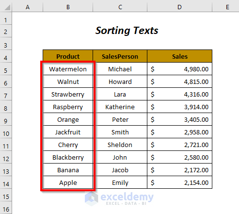
Afterward, you will get the sorted data on the basis of the Product column where the sorting appears in Descending order (From Z to A).
Read More: [Solved!] Excel Sort Not Working (2 Solutions)
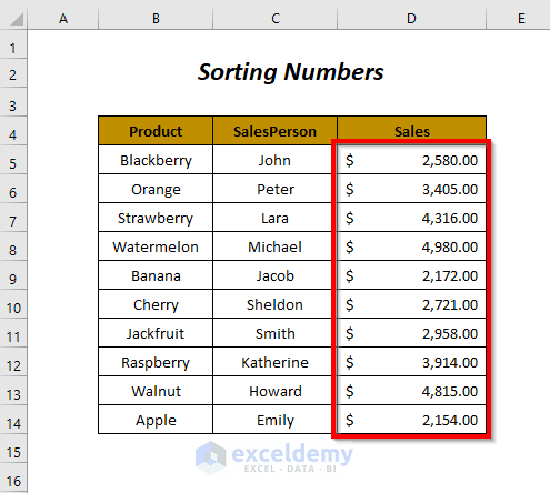
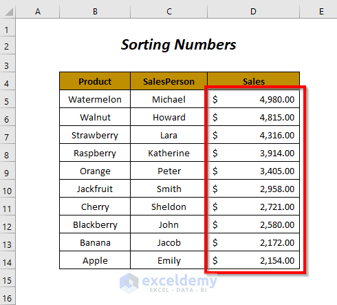
Method-2: Arranging a Group of Numbers Using Excel VBA SORT
In this section, we will arrange our data by sorting the numeric values of the Sales column.
Steps:
➤ Follow Step-01 of Method-1.
➤ Write the following code
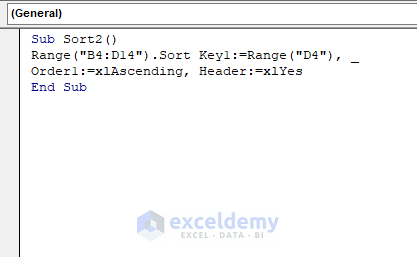
Sub Sort2()

Range("B4:D14").Sort Key1:=Range("D4"), _
Order1:=xlAscending, Header:=xlYes

End Sub
We have declared the range “B4:D14” to sort all of the values of this range and Key1 is the data range on the basis of which we are sorting our values, here it is Range(“D4”) because we want to sort on the basis of Column D, then Order1:=xlAscending indicates that the sorting order of this column will be from low value to high value and finally Header:=xlYes will determine the first row of our range as a header.
➤ Press F5.
In this way, you will get the sorted data on the basis of the Sales column where the sorting appears in Ascending order (from low value to high value).

You can sort the values from larger values to smaller values also by using the following code
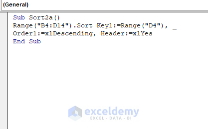
Sub Sort2a()

Range("B4:D14").Sort Key1:=Range("D4"), _
Order1:=xlDescending, Header:=xlYes

End Sub
The code is quite similar to the previous one except for Order1:=xlDescending, which means the order of the sorting process will be from a lower value to a higher value.
➤ Press F5.
Finally, you will get the sorted data on the basis of the Sales column where the sorting appears in Descending order (from higher value to lower value).
Read More: How to Sort Numbers in Excel (8 Quick Ways)
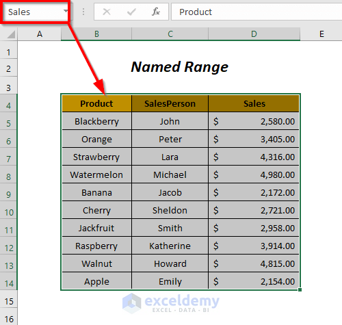
Method-3: Excel VBA SORT with Named Range
Here, we will declare our data range with the help of a named range in the VBA code and so we have named the range as Sales here.
Steps:
➤ Follow Step-01 of Method-1.
➤ Write the following code
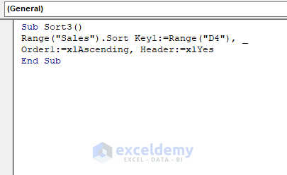
Sub Sort3()

Range("Sales").Sort Key1:=Range("D4"), _
Order1:=xlAscending, Header:=xlYes

End Sub
Here, we have used the named range “Sales” to sort all of the values of this range and Key1 is the data range on the basis of which we are sorting our values, and here it is Range(“D4”) because we want to sort on the basis of Column D, then Order1:=xlAscending indicates that the sorting order of this column will be from lower value to higher value and finally Header:=xlYes will determine the first row of our range as a header.
➤ Press F5.
After that, you will get the sorted data on the basis of the Sales column where the sorting appears in Ascending order (from smaller value to larger value).

Related Content: How to Undo Sort in Excel (3 Methods)
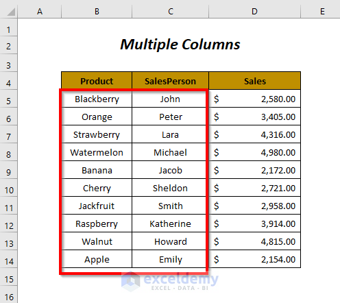
Method-4: Sorting Multiple Columns Using Excel VBA SORT Function
Here, we will sort our data range based on multiple columns like sorting the Product column in descending order and the SalesPerson column in ascending order.
Steps:
➤ Follow Step-01 of Method-1.
➤ Write the following code
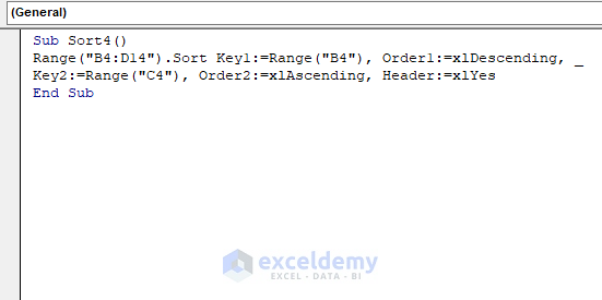
Sub Sort4()

Range("B4:D14").Sort Key1:=Range("B4"), Order1:=xlDescending, _
Key2:=Range("C4"), Order2:=xlAscending, Header:=xlYes

End Sub
We have declared the range “B4:D14” to sort all of the values of this range and Key1 is the first data range on the basis of which we are sorting our values, here it is Range(“D4”) because we want to sort on the basis of Column B, then Order1:=xlDescending indicates that the sorting order of this column will be from a higher value to lower value.
Similarly, Key2 indicates the second data range (Column C) on the basis of which we are sorting our values after the first sorting process, then Order2:=xlAscending indicates that the sorting order of this column will be from a higher value to lower value, and finally Header:=xlYes will determine the first row of our range as a header.
➤ Press F5.
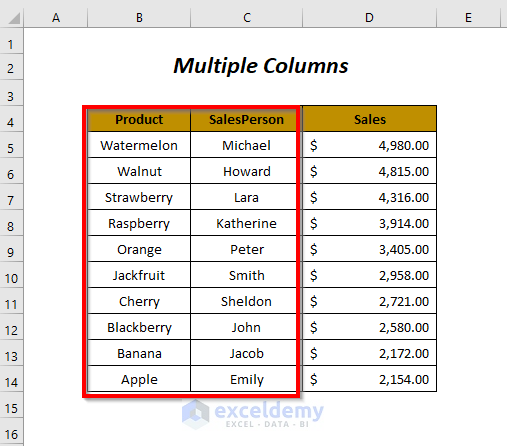
Then, you will get the sorted data on the basis of the Product column and SalesPerson column.
Read More: How to Sort Multiple Columns with Excel VBA (3 Methods)
Similar Readings:
- How to Sort Drop Down List in Excel (5 Easy Methods)
- Auto Sort Table in Excel (5 Methods)
- How to Sort ListBox with VBA in Excel (A Complete Guide)
- Sort by Month in Excel (4 Methods)
- VBA to Sort Column in Excel (4 Methods)
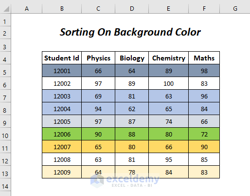
Method-5: Sorting a Group of Values-Based On Background Colour
In this section, we will sort the values on the basis of the background color of the rows.
Steps:
➤ Follow Step-01 of Method-1.
➤ Write the following code
Sub Sort5()

Worksheets("background").Sort.SortFields.Add2 Key:=Range("B5"), _
SortOn:=xlSortOnCellColor, Order:=xlAscending, DataOption:=xlSortNormal

With Worksheets("background").Sort
     .SetRange Range("B5:F13")
     .Apply
End With

End Sub
Here, “background” is the sheet name, Range(“B5”) is assigned as sort Key because we want to sort on the basis of Column B and we excluded the header row, for this reason, we didn’t have to use Header:=xlYes (by default it considers there is no header row) and moreover, SortOn:=xlSortOnCellColor is for sorting on the basis of the cell colors and the order will be from lower to a higher value.
The WITH statement helps us from the repetitive typing of the sheet name or range name or object name etc. and within this statement, we have applied the sort to the range “B5:F13”.
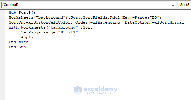
➤ Press F5.
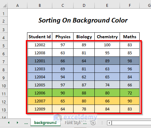
Then, you will get the sorted data on the basis of the background colors and then the Student Id column by sorting them from a lower value to a higher value.
Read More: How to Sort by Color in Excel (4 Criteria)
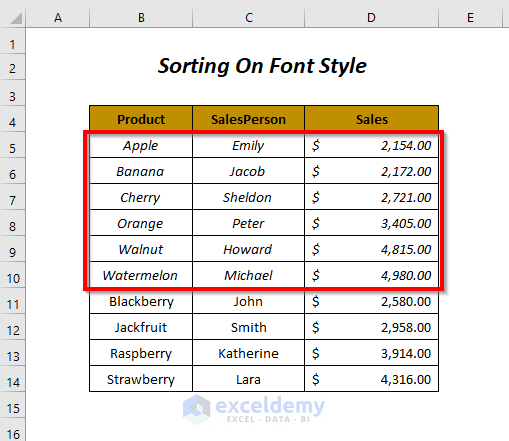
Method-6: Sorting Based On Font Style
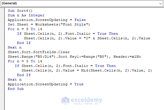
Here, we have some rows containing strings in Italic form and by using a VBA code we will sort them to the preceding positions.

Steps:
➤ Follow Step-01 of Method-1.
➤ Write the following code
Sub Sort6()

Dim n As Integer
Application.ScreenUpdating = False
Set Sheet = Worksheets("Font Style")

For n = 5 To 14
    If Sheet.Cells(n, 2).Font.Italic = True Then
        Sheet.Cells(n, 2).Value = "0" & Sheet.Cells(n, 2).Value
    End If
Next n

Sheet.Sort.SortFields.Clear
Sheet.Range("B5:D14").Sort Key1:=Range("B5"), Header:=xlNo

For n = 5 To 14
   If Sheet.Cells(n, 2).Font.Italic = True Then
       Sheet.Cells(n, 2).Value = Mid(Sheet.Cells(n, 2).Value, 2)
   End If
Next n

Application.ScreenUpdating = True

End Sub
Here, we have declared n as Integer and set it with values from 5 to 14 (the range of the row numbers), then used it with the FOR loop so that every row of the data range can be executed with the operations and set Sheet with the sheet name “Font Style”.
The first FOR loop will add 0 prior to the values of the cells in Column B only if the values are in Italic form, then Sheet.Sort.SortFields.Clear will clear all of the previous sortings and after that, we have set our sorting for the range “B5:D14” based on Column B.
After the completion of the sorting procedure, we have added another FOR loop to omit the previously added zeros by extracting the required values of the cells with the help of the MID function.
➤ Press F5.
Finally, you will get the sorted data on the basis of the font styles.
Related Content: How to Use Advanced Sorting Options in Excel
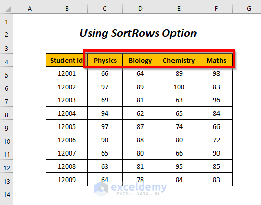
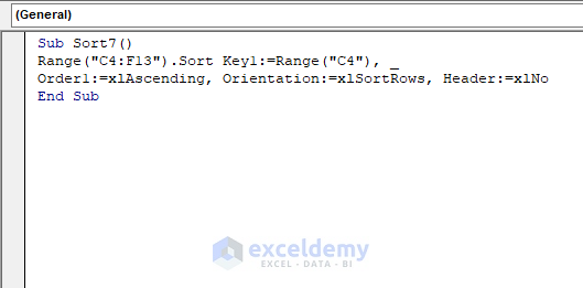
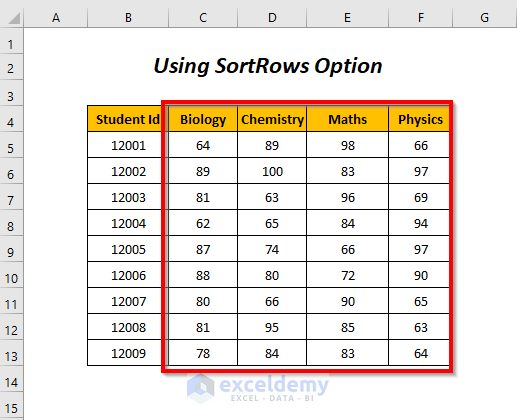
Method-7: Arranging a Group of Values in the Left to Right Direction
Typically the VBA SORT will sort the values from top to bottom, but here we will sort the marks columns from left to right on the basis of the name of subjects in ascending order.
Steps:
➤ Follow Step-01 of Method-1.
➤ Write the following code
Sub Sort7()

Range("C4:F13").Sort Key1:=Range("C4"), _
Order1:=xlAscending, Orientation:=xlSortRows, Header:=xlNo

End Sub
We have declared the range “C4:F13” to sort all of the values of this range and Key1 is the data range on the basis of which we are sorting our values, here it is Range(“C4”) because we want to sort on the basis of Row 4, then Order1:=xlAscending indicates that the sorting order of this row will be from lower value to higher value, then Orientation:=xlSortRows is for the sorting direction which is from left to right, and finally Header:=xlNo indicates that we don’t have any header.
➤ Press F5.
Afterward, you will get the sorted data on the basis of the first row in ascending order (lower value→A, higher value→Z) from left to right. So, we have arranged the Biology marks first and the Physics marks last in this way.
Related Content: Random Sort in Excel (Formulas + VBA)
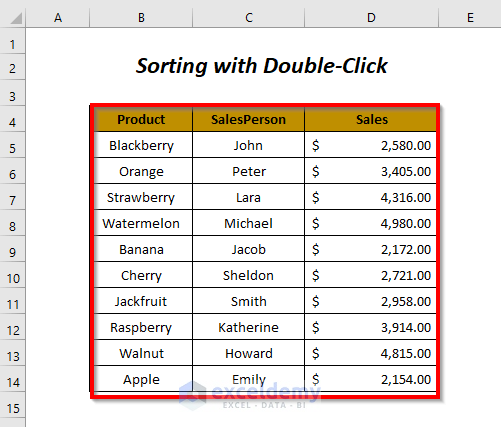
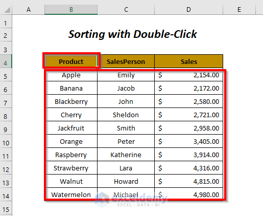
Method-8: Double-Clicking to Sort Using VBA SORT
Here, we will make our sorting procedure a little bit faster, so you have to just double-click on any of the headers and then you will get the data sorted automatically.
Steps:
You have to use the code in the right code window of the sheet on which you want to activate the double-click functionality.
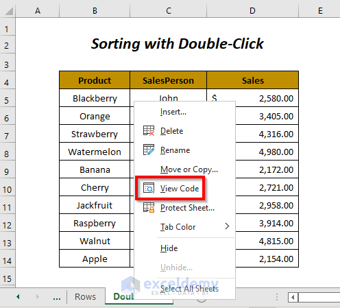
➤ Select the sheet name below the sheet and right-click on this tab.
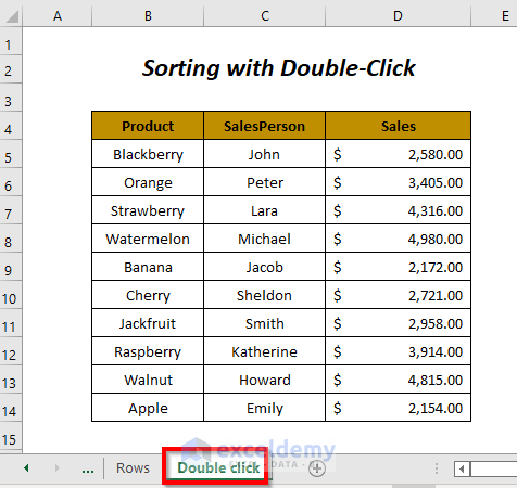
➤ Click on the View Code option.
Then, you will get a code window where you have to write the following code
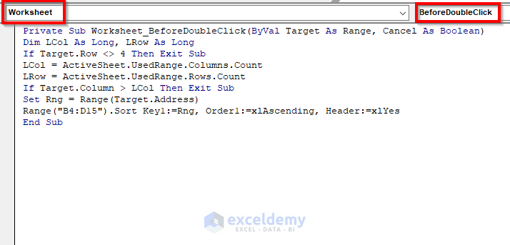
Private Sub Worksheet_BeforeDoubleClick(ByVal Target As Range, Cancel As Boolean)

Dim LCol As Long, LRow As Long

If Target.Row <> 4 Then Exit Sub
LCol = ActiveSheet.UsedRange.Columns.Count
LRow = ActiveSheet.UsedRange.Rows.Count
If Target.Column > LCol Then Exit Sub
Set Rng = Range(Target.Address)
Range("B4:D15").Sort Key1:=Rng, Order1:=xlAscending, Header:=xlYes

End Sub
The name of the subprocedure should be like this Worksheet_BeforeDoubleClick because here, Worksheet will activate the code for your sheet (you can see it in the first dropdown of the code window) and BeforeDoubleClick will activate the double click event (you can see it in the second dropdown of the code window).
We have declared LCol, LRow as Long, and they will store the column, row number of the data range.
The first IF loop will check whether the header row (Row 4 is a header row in our case) is double-clicked or not and if not then the further codes will not execute.
Then we have checked whether our selected column is inside our data range or not with the second IF loop, after that we have set Rng as the range of our selected column, and finally using this Rng we have sorted the values of the range “B4:D15”.
➤ Go back to the sheet and double-click on the header of the Product column.
Then, you will see that the values will be sorted on the basis of the Product column in ascending order.
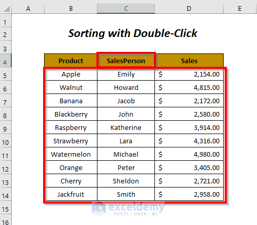
Similarly, if you double-click on the header row of the SalesPerson column, then you will see that the values will be sorted on the basis of the SalesPerson column in ascending order.
Related Content: How to Create Custom Sort in Excel (Both Creating and Using)
Practice Section
For doing practice by yourself we have provided two Practice sections like below in the sheets named Practice1 and Practice2. Please do it by yourself.
Conclusion
In this article, we tried to cover some of the ways to use the Excel VBA SORT function. Hope you will find it useful. If you have any suggestions or questions, feel free to share them in the comment section.

