How to Create Column Sparklines in Excel (5 Suitable Examples)

Get FREE Advanced Excel Exercises with Solutions!

In our everyday use of Microsoft Excel, it is important to visualize data. Sometimes it is enough to follow and measure the trend instead of going through large datasets. One of the visualization techniques Excel offers are sparklines. In this tutorial, we will focus on how to create column sparklines in Excel.

Watch Video – Create Column Sparklines in Excel

Table of Contents Expand

What Are Sparklines in Excel?

Sparklines are small, condensed charts indicating a visual representation of the trend of a range. This can fit in a cell usually and is helpful for not taking up much space. They are often used in tables, dashboards, and reports.

There are three types of sparklines available in Excel. They are:

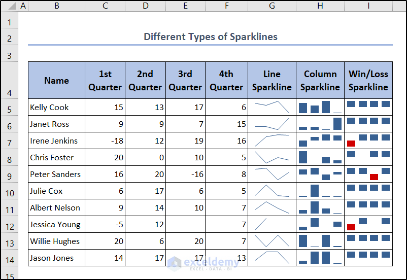
Line Sparklines: Line sparklines are tiny charts that display a row of data as a line graph. This helps to visualize the trend over a period of time.

Column Sparklines: Column sparklines are vertical bar charts that can represent the same data. They can be useful for comparing values with the magnitude of the bars.

Win/Loss Sparklines: These are also a form of column chart that shows positive and negative values. These are helpful to distinguish values that are above and below the baseline.

Read More: Types of Sparklines in Excel

How to Create Column Sparklines in Excel: 5 Suitable Examples

As we mentioned earlier, column sparklines are helpful to compare values within the range. Adding different sparkline options is available in the Insert tab. There is another method of adding sparklines using the quick analysis tool. We are going to cover how to create column sparklines in Excel for different scenarios in the following sections. For demonstration, we will be using slight variations of datasets each time for ease of understanding.

1. Create Column Sparklines for Positive Values

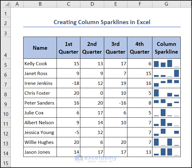
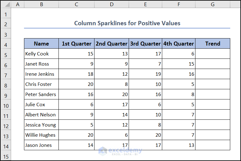
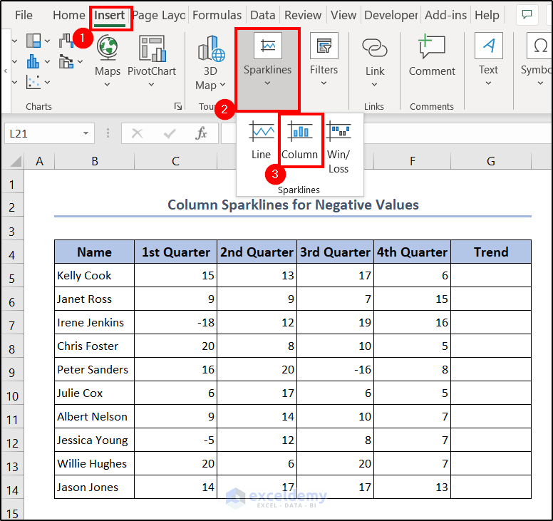
In this example, we will consider the score of 10 employees for four quarters of a year. The name of the employees is in the range of cells B5:B14. We are going to show the column sparklines in column G.

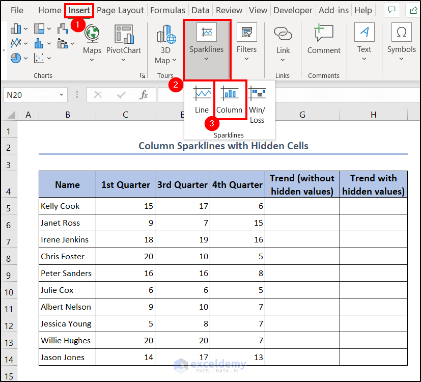
First, go to the Insert tab and select Column from the Sparklines group.

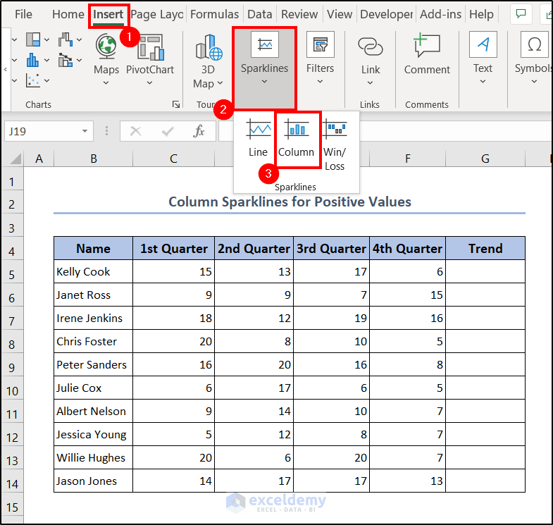
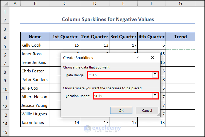
A Create Sparklines box will appear. Select C5:F5 in the Data Range and G5 as the Location Range.

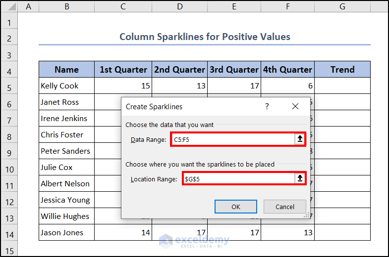
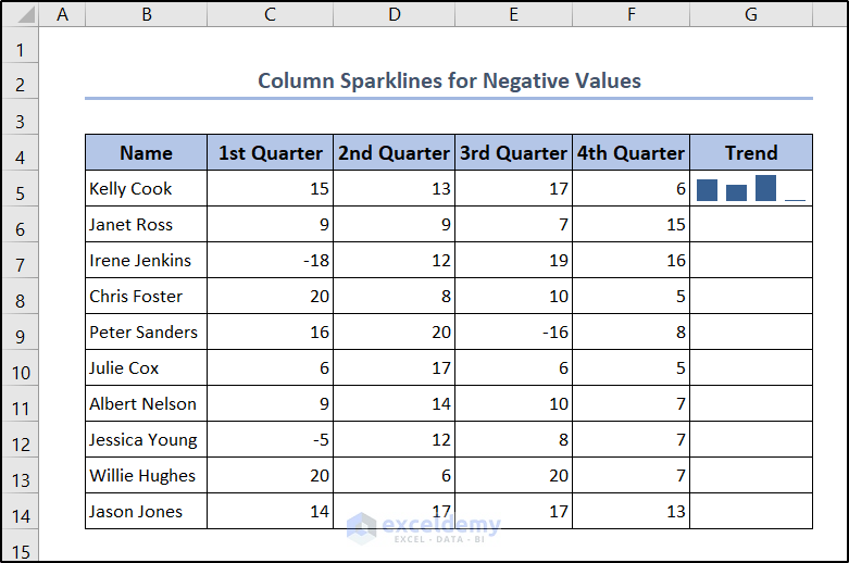
After clicking on OK, it will create column sparklines in the G5 cell of the Excel spreadsheet.

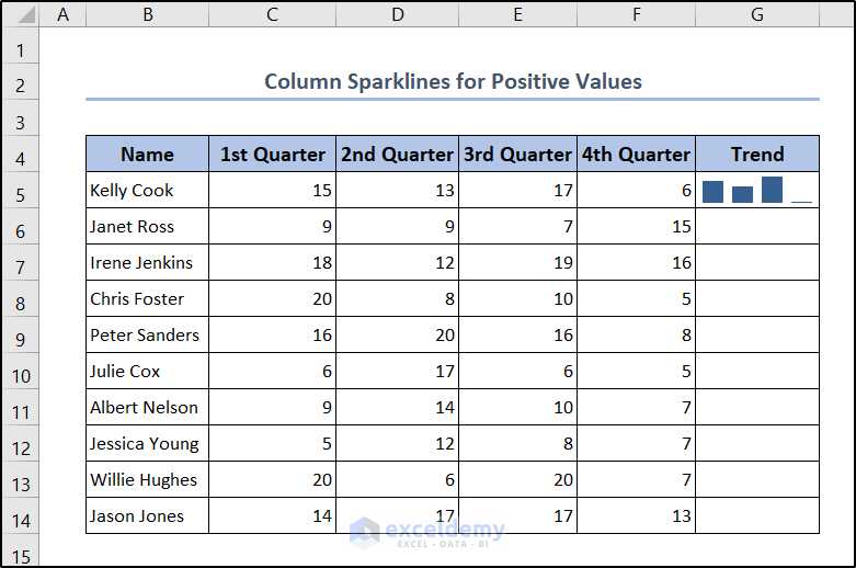
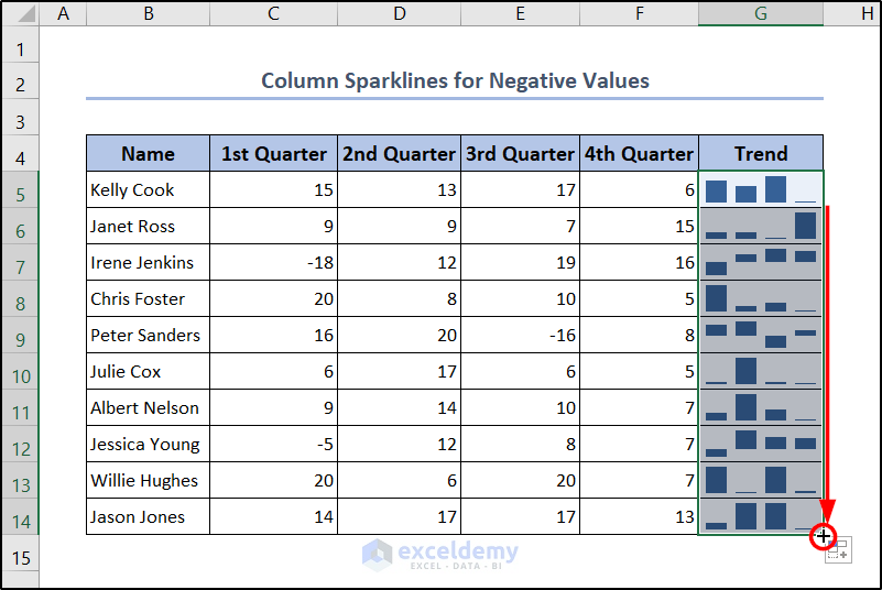
Now select the cell and drag the fill handle down to cell G14 to replicate it.

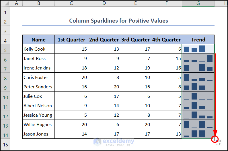
This is how we can create column sparklines in Excel very easily for positive values.

Things You Should Know

In a column sparkline, the value of the vertical axis starts from the lowest value. As a result, every lowest value in a row is close to zero.

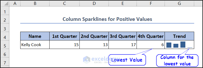
Sparkline is a light version of an Excel chart for showing the data changing pattern row-wise. It will just provide you with a preliminary idea about the data changing pattern.

Read More: How to Create Sparklines in Excel

2. Insert Column Sparklines for Zeros and Empty Values

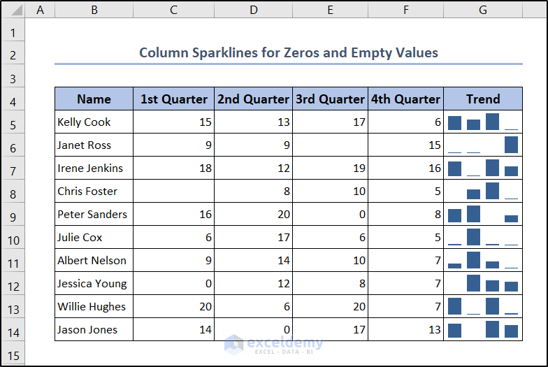
Some values in a dataset can be zero or empty. For example, some participants might have been absent or didn’t take part in the job in our dataset. Let’s take a modified version of the dataset for this.

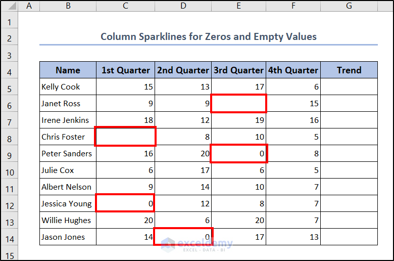
Some of the participants have blank values here and some got straight zeroes in a period. We can create column sparklines for these values in Excel too.

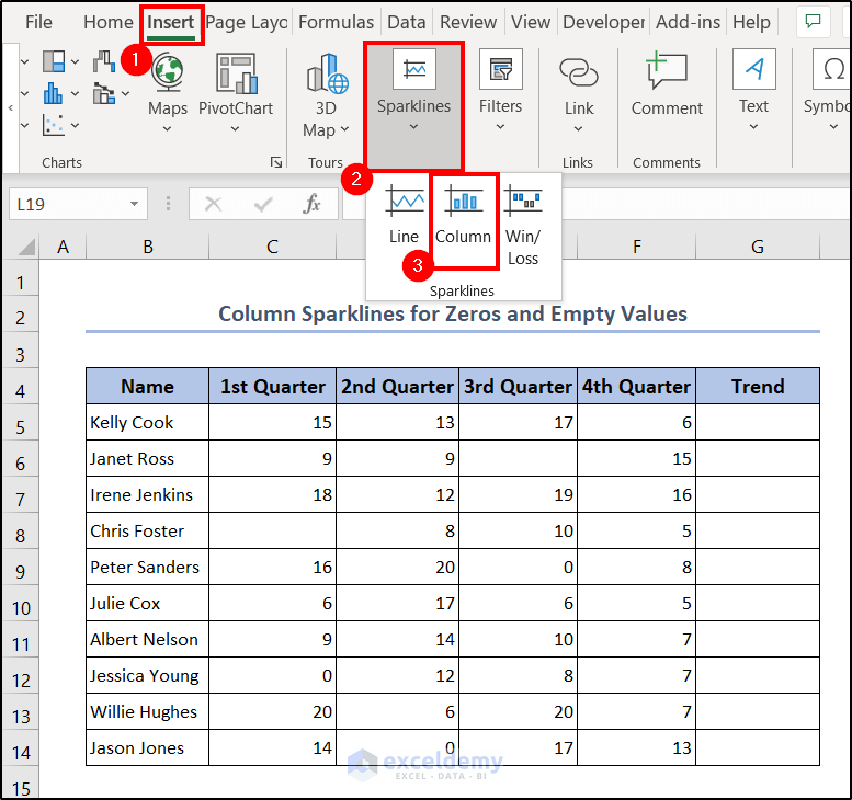
Go to the Insert tab and select Column from the Sparklines group of the tab.

Now select C5:F5 in the Data Range and $G$5 as the Location Range in the Create Sparklines box.

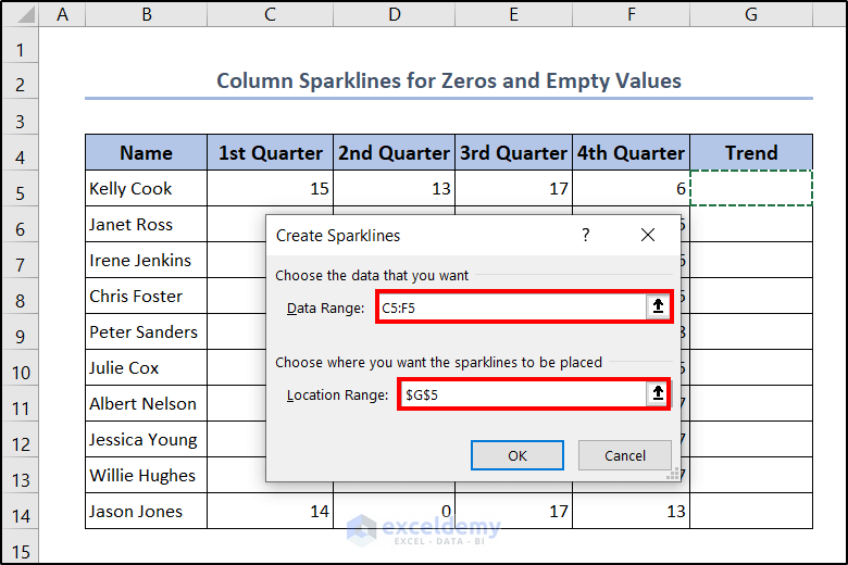
As you click on OK, you will get the column sparklines in the G5 cell.

Selecting the cell again and dragging the fill handle down to cell G14 will give the column sparklines for the rest of the cells.

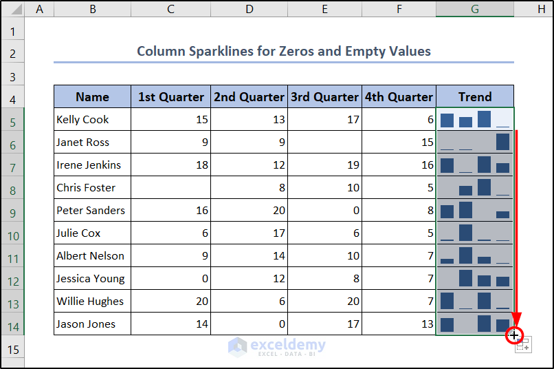
As we can see, we can follow the same procedure to create column sparklines in Excel for zeroes and empty values.

Interpretation of the Sparklines

You may notice that the column sparklines pattern at the rows of 0 value and empty cells are not similar to the other rows.

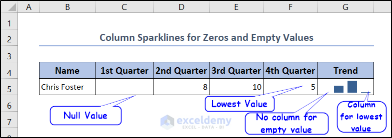
If we consider an empty row from the dataset, we can see the first value here is empty and the last value is the lowest value. In the sparkline, there is a space for a column but nothing there for the empty value. For the lowest value, there is a slight mark of column proportional to other values.

Dealing with Zero Values

There are two types of column sparklines when there are zero or empty values in it. The one we previously created is where Excel considers a gap in the case of zero values and the rest of the cells adjust according to the non-zero values. There is another way to show the sparklines- adjusting non-zero values based on taking the gaps as zeroes.

To consider the empty values as zero and start the baseline from there, follow these steps.

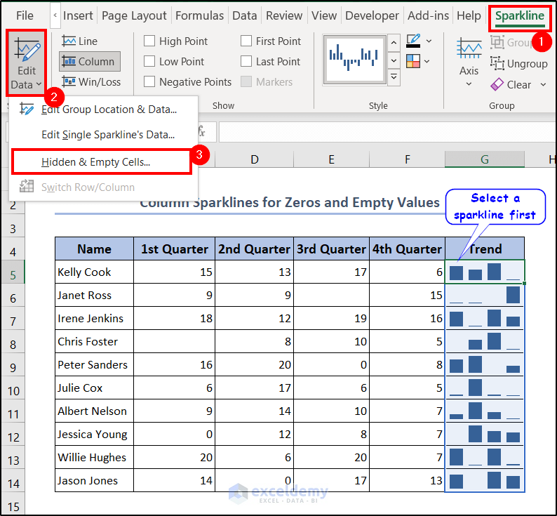
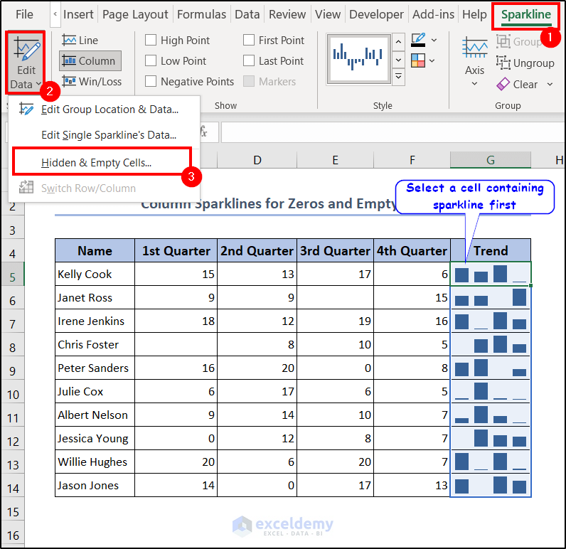
Select a sparkline cell and the Sparkline tab will appear on the ribbon.
Go to the tab and select Edit Data.
From the drop-down list, select Hidden & Empty Cells.

In the Hidden and Empty Cell Settings, select Zero as the Show empty cells as option and click on OK.

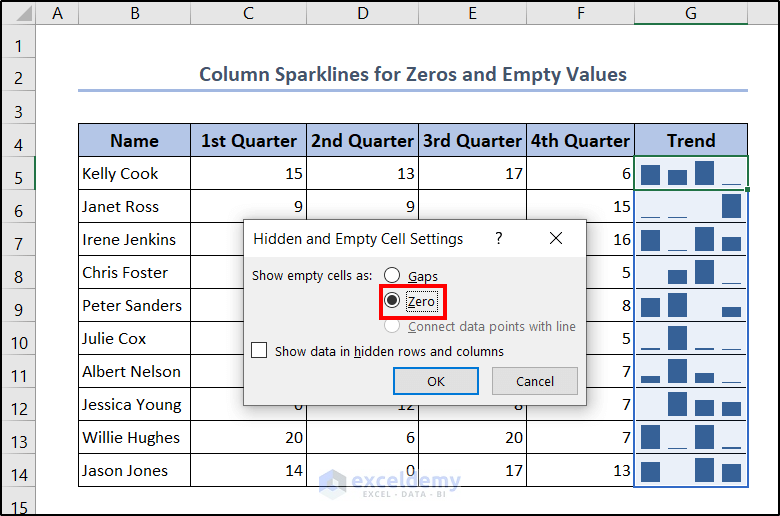
As a result, Excel will include the empty and zero values and rearrange the columns starting from zero.

To revert them back to gaps, follow these steps.

First, select a cell containing a column sparkline and go to the Sparkline tab that will appear on the ribbon.
Select Edit Data and then Hidden & Empty Cells from the drop-down list.

In the Hidden and Empty Cell Settings box, select Gaps as the Show empty cells as option.

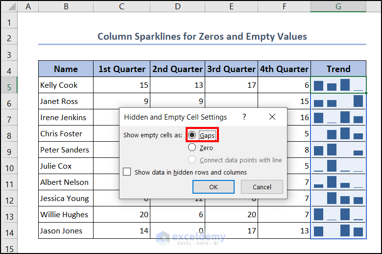
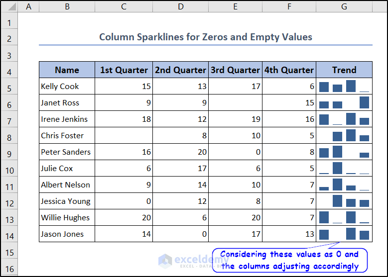
After clicking on OK, the sparklines will rearrange in such a way that the empty values are gaps but the rest of the columns are rearranged ignoring the zero value. It is now starting from the lowest point.

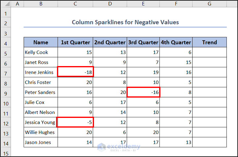
3. Create Column Sparklines for Negative Values

We can create column sparklines in Excel for negative values in the same way too. In a sense, it is similar to the win/loss sparklines.

However, the column sparklines with negative values have a height according to the magnitude of the value. At the same time, the win/loss sparklines have either an upward or downward value regardless of the amplitude of the value.

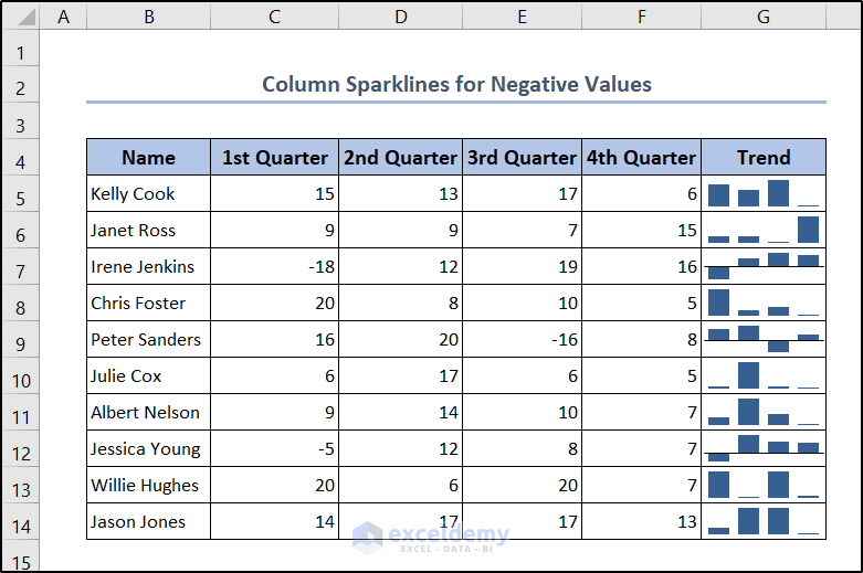
Let’s rearrange our dataset to have some negative values as we can see from the following figure. This is very common in the case of negative scoring.

Go to the Insert tab on the ribbon and select Column from the Sparklines group.

Then select C5:F5 as the Data Range and $G$5 as the Location Range in the Create Sparklines box.

After clicking on OK, you will get the sparkline for the first row.

Now select cell G5 and drag the fill handle down to the end of the column to create sparklines for the rest of the cells in the Excel spreadsheet.

To show the axis in the sparkline that better represents the regular value, select a cell and go to the Sparkline Select Axis and Show Axis from the drop-down menu.

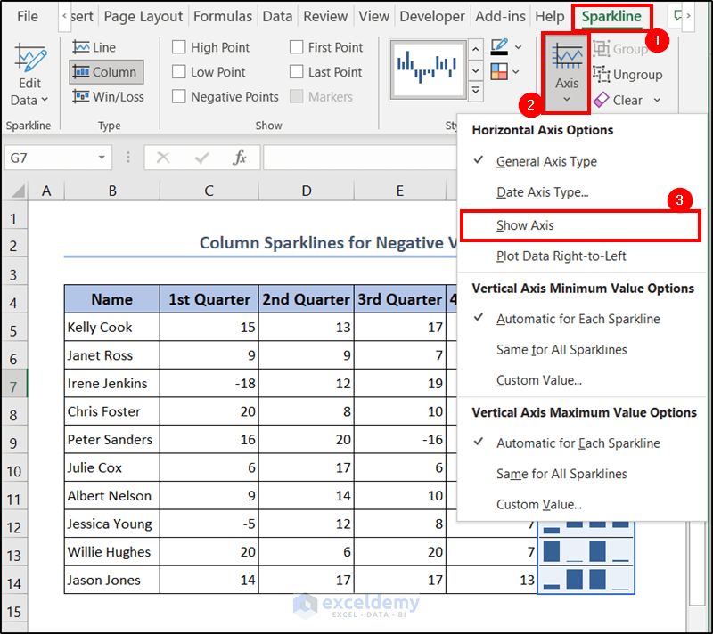
The final result will show sparklines with a black baseline that shows which columns are above and which are below indicating positive and negative values.

Interpretation of the Result

Let’s take a row from the dataset.

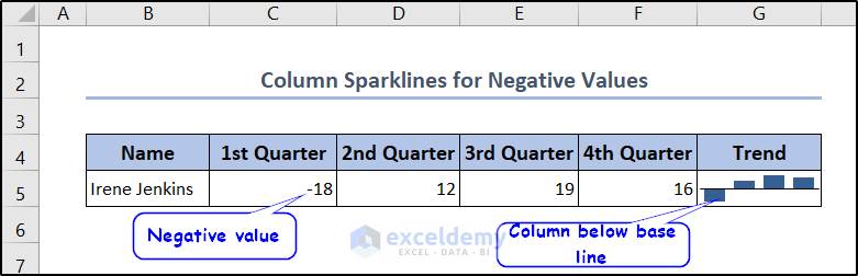
As we can see the score from the 1st quarter is negative in the range. In the column sparkline cell, we can see the first column is downward in direction. This indicates the negative value of the range. The rest of the cells are above the baseline indicating positive values and the third one is the highest in height indicating the highest value in the third cell of the range.

4. Create Column Sparklines with Hidden Cells

We sometimes hide columns or rows in a spreadsheet to focus on relevant data, protect sensitive information, create print-friendly layouts, etc. This is a handy feature for those purposes. But while creating sparklines, Excel treats hidden and unhidden ranges differently.

For example, let’s take the original dataset. But this time, the scores of the 2nd quarter (column D) are hidden.

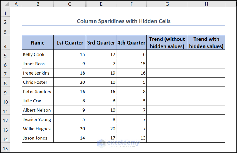
Now let’s create column sparklines to visualize how it is with and without the hidden column values.

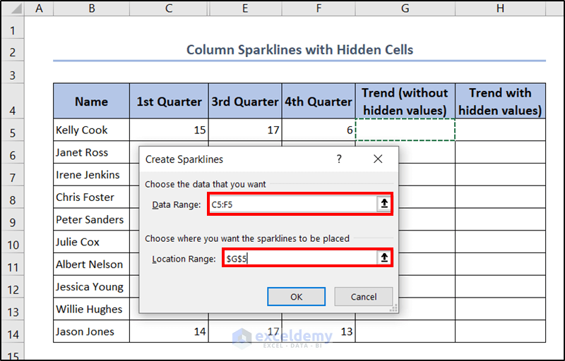
Go to the Insert tab and select Column from the Sparklines group.

In the Create Sparklines box, select C5:F5 as the Data Range and $G$5 as the Location Range.

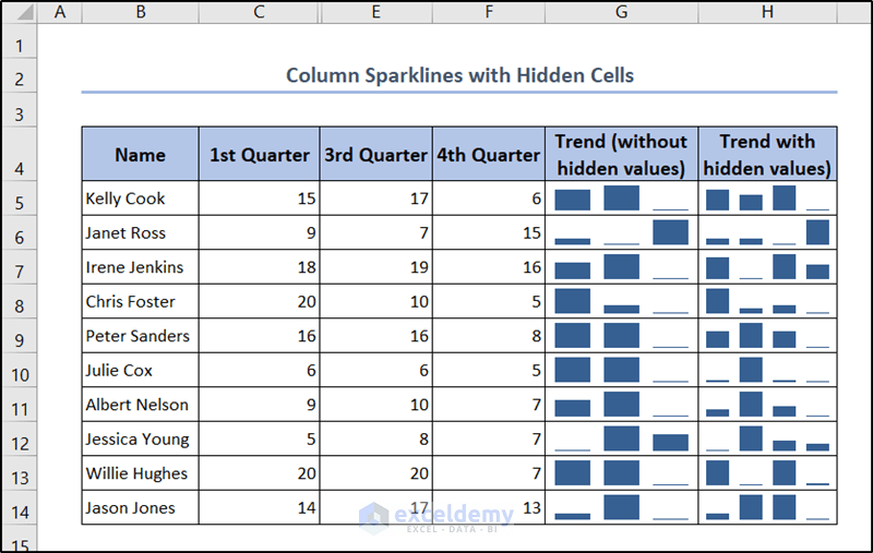
After clicking on OK, we can get the column sparklines for the first row. We can drag the fill handle down to create the sparklines for the rest of the rows.

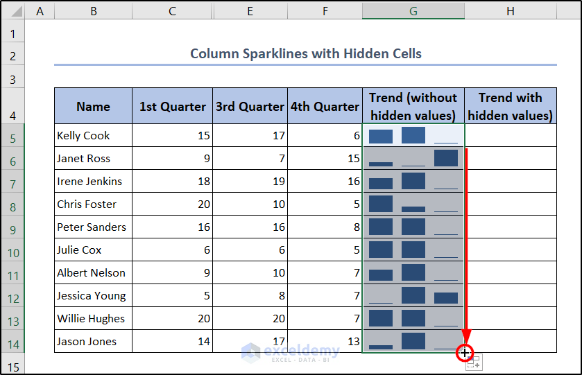
We can see from the figure above, there are three columns in the sparklines. This is because a column is hidden and sparklines are developing based on the columns that are showing.

What If I Want to Show Hidden Values When Creating Column Sparklines?

There are ways to work around it to have the hidden values appear on the sparklines. Follow these steps to do that.

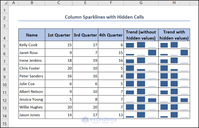
First, create column sparklines with the steps described above. We are inserting them in the range H5:H14.

Now select a cell in the range and go to the Sparklines tab that appears after selection.
Select Edit Data there and select Hidden & Empty Cells from the drop-down.

Now check the Show data in hidden rows and columns in Hidden and Empty Cell Settings that popped up.

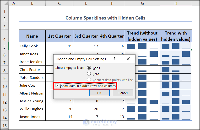
After clicking OK, you will see that the hidden values are now included in the column sparklines.

5. Create Column Sparklines Using Quick Analysis Tool

The Quick Analysis Tool is a feature available in Excel that provides convenient ways to explore, visualize, and format data. This is the icon that appears at the end when you select a range of cells. We can use it to create column sparklines in Excel easily too. For example, let’s take the original dataset and insert column sparklines using this method.

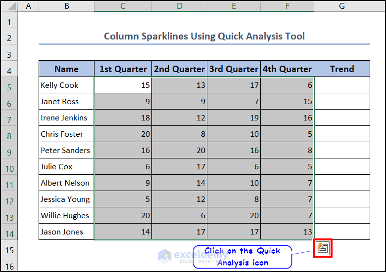
First, select the whole range containing data. In our case, the range is C5:F14.
Then click on the Quick Analysis icon that appears at the bottom-right of the selection.

Now select Column from the Sparklines section in the window.

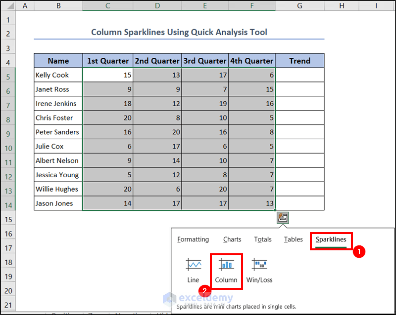
This will create column sparklines for all the cells in the Excel spreadsheet.

How to Change Sparklines Type in Excel

You may often create a type of sparkline and find out that it does not align with your purpose. So it may be very common that we have to change the sparklines we have created up to a point. However, we don’t need to delete the sparklines and start all over after creating one.

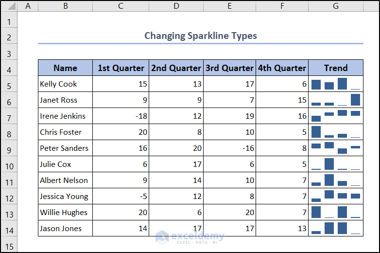
Let’s take the following dataset we have already created.

To change the sparklines type, select a cell containing the sparklines and go to the Sparklines tab that appears after selection.
In the Type group, you will find the other types of sparklines available.

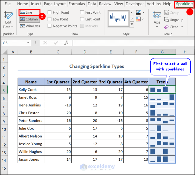
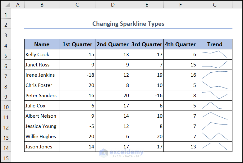
Choose Line to get the Line Sparklines.

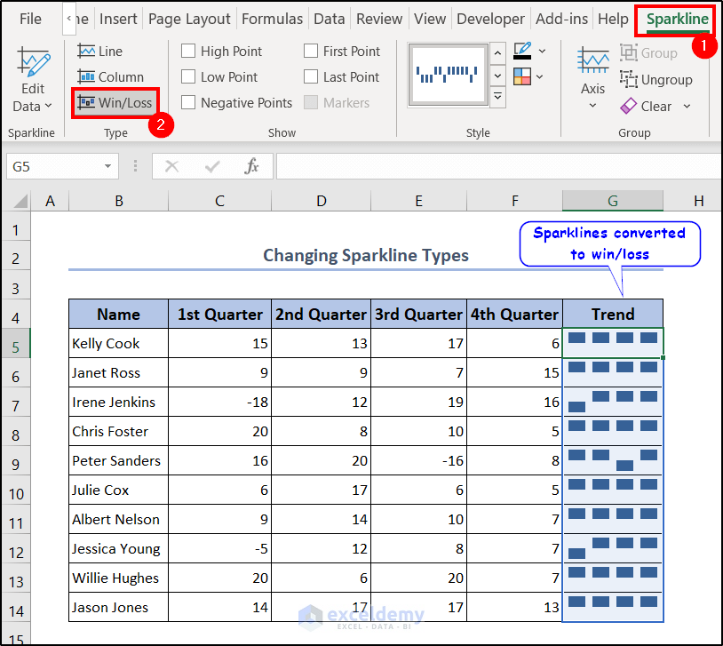
If we choose Win/Loss, we will get a win/loss sparkline.

How to Select Same Axis for All Sparklines in Excel

Each of the sparklines we create has different axes by default. But we can also change that to be the same in a range.

Select a cell in the range containing sparklines.
Then go to the Sparkline tab and click on Axis.
From the drop-down menu, select Same for All Sparklines under both Vertical Axis Minimum Value Options and Vertical Axis Maximum Value Options.

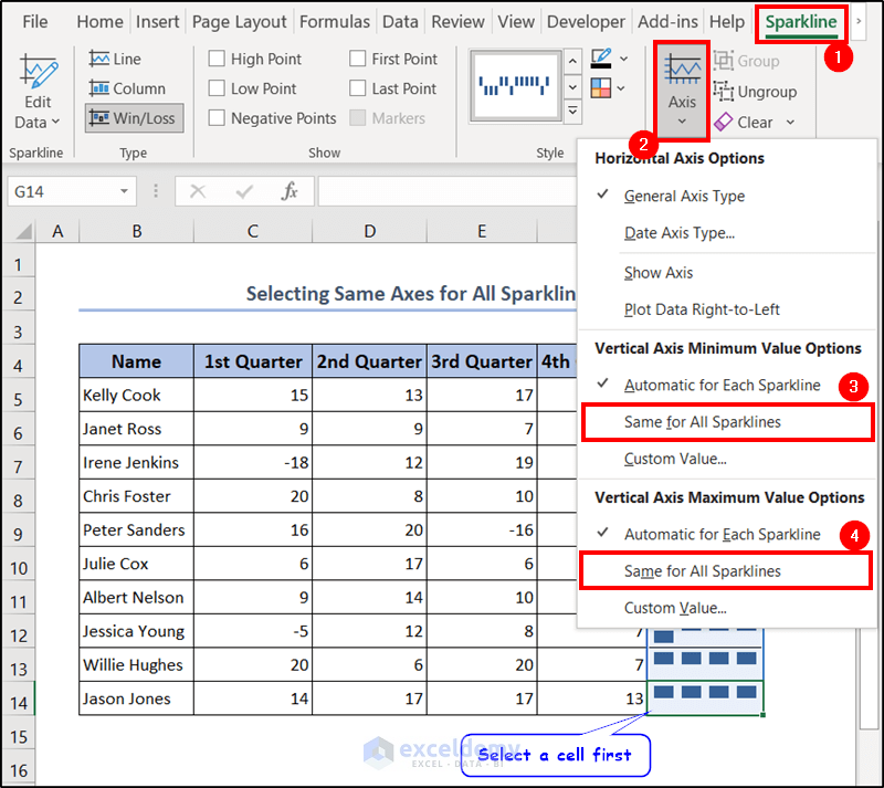
This will reset the minimum value of all sparklines to the same and thus they will have the same axis.

Things to Remember

The sparkline feature is available in Excel 2010 or later only.
If a range of sparklines is not grouped, changes from the Sparkline tab are only applicable to the selected cell.
For column sparklines, the negative and positive values have different heights. But for win/loss sparklines they have the same height regardless of the value.
Sparklines are always dynamic in nature. They always change automatically if the cell range or value changes.
We can follow the same steps to create sparklines in Excel Table or Pivot Table too.
You can not delete a sparkline by using the Delete button like other cell values. Instead, use the Clear All command for that.

Frequently Asked Questions

1. How to group/ungroup Sparklines in Excel?

To group/ungroup any kind of sparklines, select a cell/the range(in case of grouping) and go to the Sparkline tab. There you will find the Group/Ungroup option in the Group group.

2. How to Delete Sparklines in Excel?

To delete a sparkline from a cell/range of cells, select them and select Clear. You will find it in the Home tab’s Editing group. You need to select Clear All from the drop-down to delete the sparklines. It will remove all the values and formats of the cell.

3. How do I customize sparklines in Excel?

The Show and Stype groups are available in the Sparkline tab. This tab appears once you click on a cell that contains a sparkline. You can use the options in the groups to customize sparklines within Excel.

Download Practice Workbook

You can download the workbook used for the demonstration from the link below.

Create Column Sparklines.xlsx

Conclusion

That concludes our discussion on how to create column sparklines in Excel. We have covered different types of data while creating column sparklines. We have discussed how hidden columns/rows interact with column sparklines. To insert column sparklines, we have both used the Insert command and the Quick Access Tool. Hopefully, you can create column sparklines for your dataset pretty quickly and easily too. I hope you found this guide helpful and informative. If you have any questions or suggestions, let us know in the comments below.

<< Go Back to Excel Sparklines | Learn Excel