Latest Posts From Mahfuza Anika Era

In this article, I have described what DAX is in Power Pivot and how to use it, including its applications and benefits. I have shown the use of three ...

In this Excel tutorial, you will learn how to -Create a thermometer chart/goal thermometer -Create a twin thermometer chart We have used Microsoft 365 to ...

In this Excel tutorial, you will learn how to - Check the encoding of an Excel file - Change the encoding to UTF-8 using the web option - Change the ...

Commas in Excel can sometimes be an obstacle when working with numerical data or text strings. Fortunately, Excel provides several methods to remove commas ...

In this Excel tutorial, you will learn how to - Delete a sheet in Excel - Delete multiple sheets - Use VBA to delete sheets We have used Microsoft 365 to ...

In Excel, we use the Freeze Panes feature to lock or fix specific rows or columns in your worksheet so that they remain visible as we scroll through the rest ...
In this article, I have illustrated 25 powerful techniques and features of PivotTable. I have mostly covered advanced levels of Pivot Table in Excel. If you ...

Returning all rows that match criteria in Excel means showing the rows in a dataset that meet specific conditions. In this Excel tutorial, you will learn ...

If you want to comment on multiple lines in a VBA code to make the code easily understandable, this article can help you to do this in 3 simple steps. ...

Date Picker is a type of calendar from which you can navigate through the months and years and insert the date into the cell. In an Excel UserForm, a date ...

Remembering long Workbook names takes extra time and effort. Using VBA, you can activate a Workbook without remembering its full name. Isn’t it great? With the ...

Are you trying to exit a Select Case Statement for a specific condition in Excel VBA? It greatly helps to optimize the performance of the code. Unfortunately, ...

Are you trying to move the X-axis of your Excel chart to the bottom? There are so many cases where you need to place the X-axis or horizontal axis at the ...

Are you looking for an Excel function that will return the standard deviation of the entire population and also match the given criteria? In this case, the ...

Looking for ways to create InputBox with password mask in Excel VBA? Then, this is the right place for you. To prevent shoulder spying, you should use a ...


Hello MARIANOLI,
Thank you so much for your comment. You can fix this problem by changing the date format in your computer’s date and time settings. Change the date format to dd/MM/yy. Hopefully, you will get the dd/mm/yy format for the whole month.
Regards
Mahfuza Anika Era
ExcelDemy
Dear NURIT,
Thank you so much for your comment. I have changed the date format to United States format in the code. You have to change the VBA code in the subroutine named Private Sub Create_Calender(). Following is the code for your required date format.
Here is the screenshot of the new code. I have marked the changes for your better understanding.
Regards
Mahfuza Anika Era
ExcelDemy
Dear Ahmad,
Thanks for your query.
In the VLOOKUP function #N/A error occurs when you type the wrong lookup value or worksheet name. So, check if you have given the lookup value and worksheet name properly.
Again, VLOOKUP can only look up values to the right of the lookup value. Be careful about this.
If you need further help, please mention details about your problem.
Regards
Mahfuza Anika Era
ExcelDemy
Dear Salad,
Thanks for your question. Here is the VBA code that will give you your mentioned output.
Following is the output after using the code.
Regards
Mahfuza Anika Era
ExcelDemy
Dear MARK,
Thank you for your query.
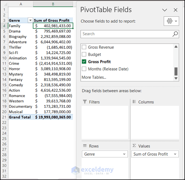
Here is the dataset I will use to show the solution to your problem.
After creating a PivotTable, I have copied the PivotTable 5 times. So, there are 5 PivotTables in my worksheet now.
Now, we have to create a drop-down menu from the list of PivotTables.
Next, copy this VBA code into your VBA code editor. You have to change three things in this code. These are: the cell address of where you placed the drop-down menu, the filter values, and the field name that you want to filter.
To get the output, select the PivotTable from the drop-down which you want to filter, and then Run the code by pressing the F5 key.
For your convenience, I have given the Excel file: Filtering PivotTable with drop-down menu.xlsm
Regards
Mahfuza Anika Era
ExcelDemy
Dear Stuart,
I am glad that you find this article informative. Thank you for your query. The VBA code which I have inserted in step 4 is in Sheet1 under Microsoft Excel Objects Section.
Mahfuza Anika Era
ExcelDemy
Dear Yosh,


Thank you for your query. Yes, you can determine the sum of YTD number. Firstly create a table like the following for each Month’s Sales of “Jimmy” for “Laptop”.
Copy this formula in cell C21.
=SUMIFS(INDEX($D$5:$I$16,,MATCH(B21,$D$4:$I$4,0)),$B$5:$B$16,$B$20,$C$5:$C$16,C$20)You will get the sales for each month.
Next, to calculate the “YTD Grandtotal” copy this formula in cell C27.
=SUM(C21:C26)I hope this method will solve your problem. Thank you!
Mahfuza Anika Era
ExcelDemy
Dear Yosh,
I assume, this question is same as the previous one. You can follow the steps I have given in the previous reply. If you still have any confusion, please leave a comment describing your problem. Thank you!
Mahfuza Anika Era
ExcelDemy
Dear L,
Thank you for your comment. This formula calculates a date value. Here is a breakdown of what each part of the formula does:
=$B$4-(WEEKDAY(C$3,1)-($AM$7-1))-IF((WEEKDAY($B$4,1)-($AM$7-1))<=0,7,0)+1
$B$4: This is the reference to cell B4 which contains the date value you enter in Customize Dates Table.
WEEKDAY(C$3,1): This function calculates the weekday of the date in cell C3. The argument 1 specifies that the weekday numbering should start on Monday (1) instead of Sunday (default value of 0).
$AM$7: This is a reference to the cell containing a number that specifies the Start Month. (e.g. 1 for Monday, 7 for Sunday).
IF((WEEKDAY($B$4,1)-($AM$7-1))<=0,7,0): This function checks whether the weekday of the date in cell B4 is earlier in the week than the specified start day of the week. If it is, the function returns 7 (the number of days in a week) to adjust the date calculation later. If not, the function returns 0.
B4-(WEEKDAY(C3,1)-($AM$7-1))-IF((WEEKDAY($B$4,1)-($AM$7-1))<=0,7,0)+1: This formula subtracts the weekday of the date in cell C3 from the date in cell B4, then adds the start day of the week minus 1, and finally subtracts the result of the IF function. This calculates the first day of the week that contains the date in cell B4. The final +1 adds one day to get the actual start date of the week.
If you want 4 weeks in one sheet, just add 3 more weeks similarly in the existing sheet. Hope this will help you.
Regards
Mahfuza Anika Era
ExcelDemy
Dear Max,
Thank you for your query. Changing the currency is not the reason behind the incorrect output of the module 2 code. Actually, the code is not working for the last 3 digits of the whole number part. Here is the modified code of module 1 that may help you. This will give the correct result hopefully.
Copy the code in your module and Run the code.
I hope you have got your problem solved. Thank you.
Regards
Mahfuza Anika Era
ExcelDemy