Formatting Tool in Excel (Tool Types & Uses)

Get FREE Advanced Excel Exercises with Solutions!

In this article, we will learn about all the formatting tool in Excel. Formatting tools in Excel help us to format the cells as well as the worksheet and help us to visualize the data more effectively. We can also protect our data using these formatting tools.

Here we will learn how to format the cells using the Format Cells dialog box. Formatting includes changing the number type, applying fill color, and Changing the font type, style, size, and color. We can also apply different types of borders to make the worksheet more organized.

Also, we can do these changes using the Excel ribbon’s Home tab. We will learn about the processes in this article. Excel charts are also important in terms of data analysis. So formatting an Excel chart is also an important task to make it more understandable. We will also learn the process to format a chart in this article.

Download the Practice Workbook

Formatting Tool.xlsx

Table of Contents Expand

How to Use Formatting Tool in Excel

1. Using Format Cells Dialog Box

Here we will learn to format cells using the Format Cells Dialog box. To open this dialog box, press Ctrl+1 on your keyboard.

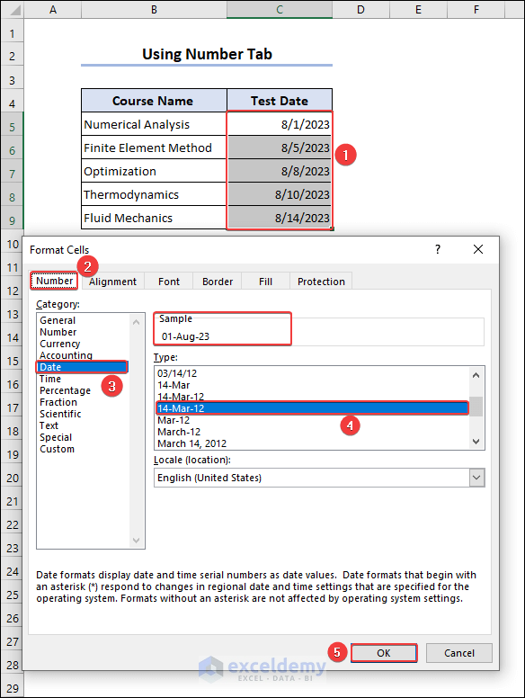
1.1 Using Number Tab to Change Data Type

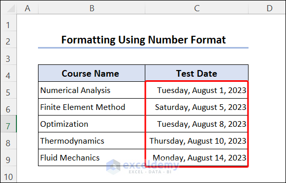
To format cells using the Number tab from the Format Cells dialog box, select the cells C5:C9 and press Ctrl+1 on your keyboard.
Then go to the Number tab and choose Date from the Category options. Then select any date format and click on the Ok button.

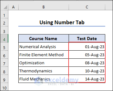
Now we can see that the date format has changed.

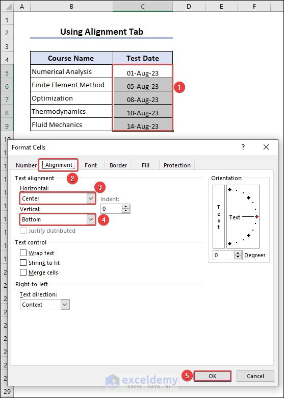
1.2. Working with Alignment Tab to Change Data Alignment

In the Alignment tab, we can change the alignment of the text in a cell.
To do this select the dataset then press Ctrl+1. From the Format Cells dialog box, go to the Alignment tab.
From the Horizontal and Vertical dropdown options, you can choose a suitable alignment for you. Here we chose General for Horizontal and Center for Vertical Alignment.

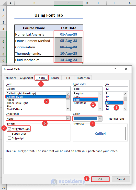
1.3. Changing Fonts from Font Tab

In the Font tab of the Format Cells dialog box, we can change the Font, Font style, Size, Color, Effects etc. Here we selected the following options shown in the image below and clicked on the Ok button. And we can see how it changed the dataset.

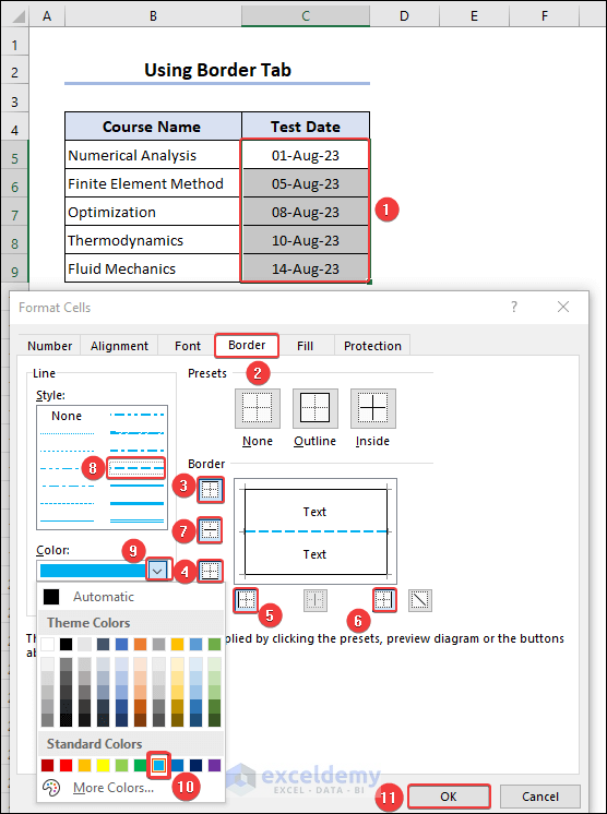
1.4. Applying Borders with Border tab

We can change the border type using the Format Cells dialog box.
Select cells C5:C9 and press ctrl+1. Go to the Border tab, then select border style. Then select the borders.
Here, we can customize border styles and colors for each border. In this case, we have to select the border that we want to change and then apply styles. In this example, we have customized the middle borders of the selection range.
After selecting and customizing borders, click the OK button.

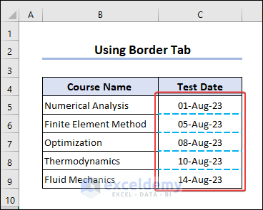
Now we can see that the border style has changed.

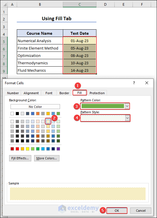
1.5. Using Fill Tab to Change Cell Background Fill

We can also fill the background of the cell using the Format Cells dialogue box.
To do this select the data range. Press ctrl+1 to open the Format Cells dialog box.
From there, go to the Fill tab. Choose the Background Color, Pattern Color, and Pattern Style according to your use. Then click OK.

1.6. Protecting Cells/ Sheets with Protection Tab

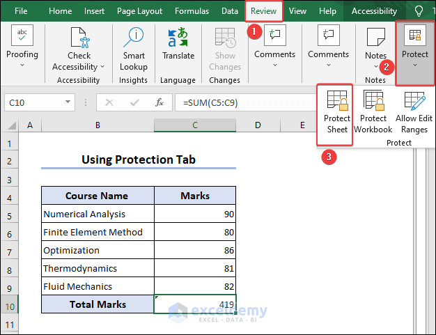
First, select the cell that contains the formula. Then press ctrl+1 and from the Format Cells dialog box go to the Protection tab. From there choose Hidden. This will hide the formula.

Then go to Review >> Protect >> Protect Sheet.

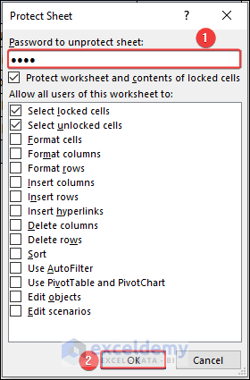
Then give a password and click OK.

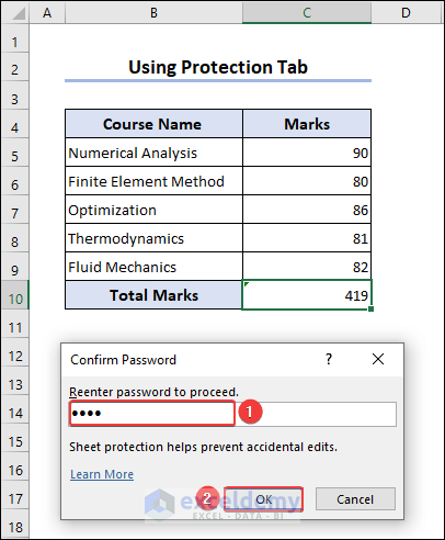
Re-enter the Password and click OK.

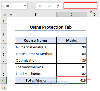
Now if we click on the cell, we will see the formula is hidden.

2. Recycling Excel File Formats

In this method, we will learn to copy a format and then paste it into a different place.

2.1. Copying over Formats

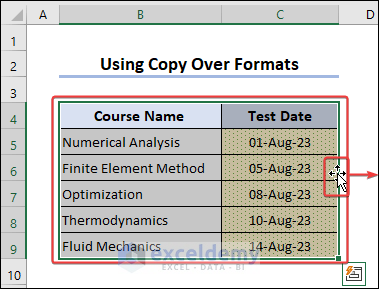
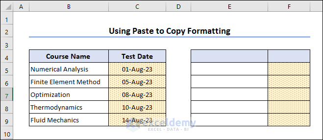
First, select the dataset whose format you want to copy. Then move the cursor at the end of the dataset. When the Move cursor appears, Left-click the mouse and drag it to the place where you want to paste it.

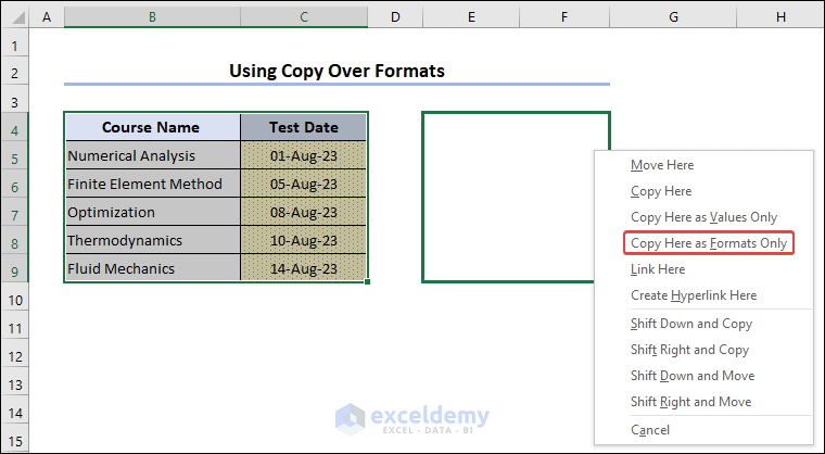
Here we dragged it to cell E5:F9. Then release the left-click and then a context menu will open. Click on “Copy Here as Formats Only” option.

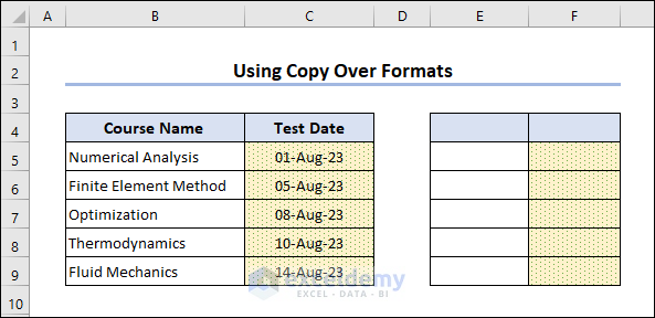
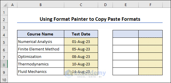
Finally, we can see only the format of the dataset has been copied and pasted.

2.2. Using Formatting(R) Options from Paste Special

Now we will use the paste options to copy formats. To do this select the dataset and press Ctrl+C to copy. Then select the destination cell and Right-click the mouse. Then a context menu will open. From the Paste Options, select Formatting (R).

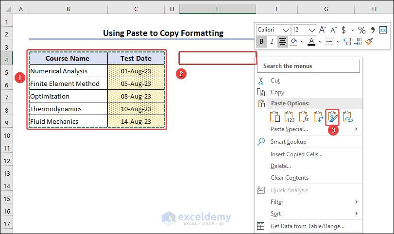
This will only paste the format of the copied dataset.

3. Using Excel Ribbon’s Home Tab

Now we will use the Excel ribbon’s Home tab options to format cells.

3.1. Using Clipboard Group to Copy and Paste Formats

Copy and Paste Options:

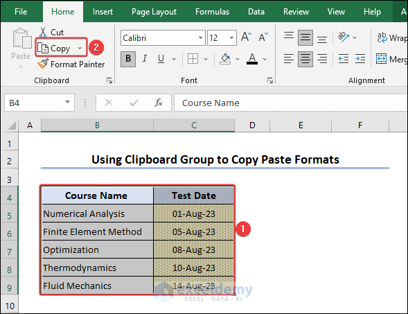
In the clipboard group, we can see there are multiple options. In this method, we will only use the Copy and Paste options to copy and paste formats.
First, select the dataset then click on Copy.

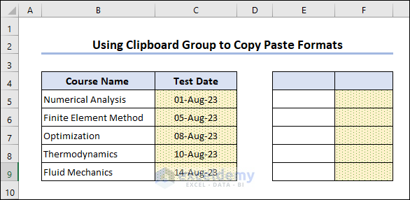
Then, select the destination cell and from the ribbon select Paste >> Other Paste Options >> Formatting (R).

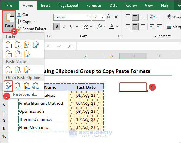
Then we can see only the format of the dataset in the destination cell.

Format Painter Tool:

We can also copy formats using the Format Painter option from the Clipboard group. Select the dataset click on Format Painter and click the destination cell (cell E4 here) where we want to paste the format.

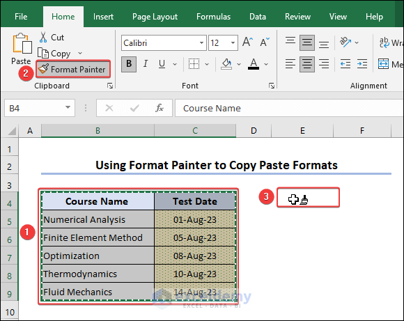
Using this method we can only paste the format of the dataset and reuse it.

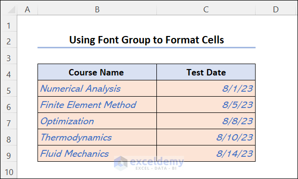
3.2. Using Font Group to Format Cells

Now we will learn to change the format using the Font Group.

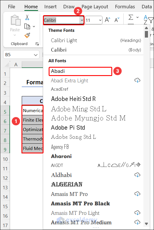
Font Changing:

We can change the font type from the Home Tab. First, select the dataset then go to the Font group from the drop-down menu and select the font type suitable for you. Here we have changed our font from Calibri to Abadi.

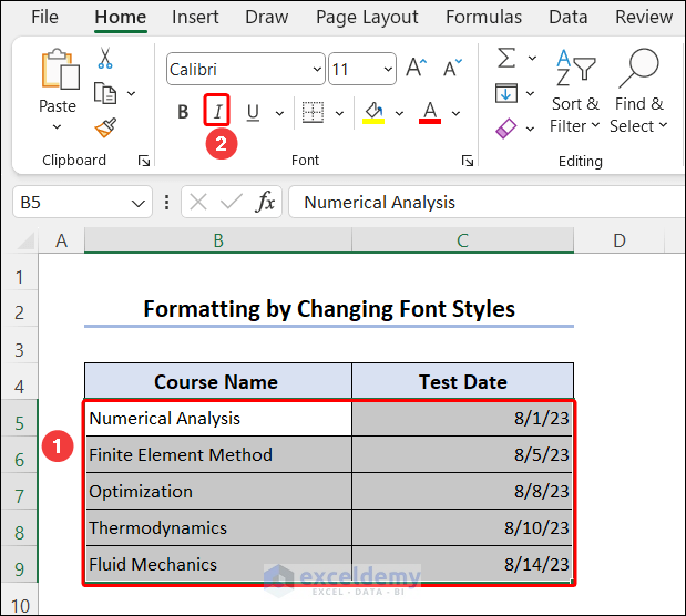
Changing Font Style:

The font style includes Bold, Italic, and Underline. Here we will change the font style to Italic. For this, select the dataset and choose Italic from the Font group.

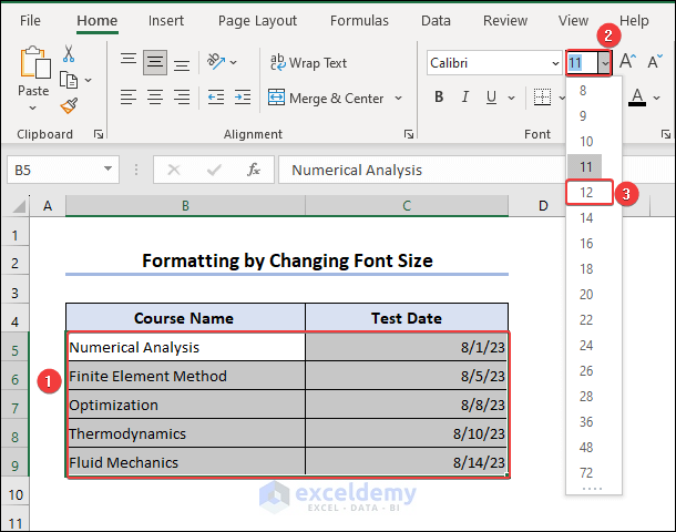
Font Size Changing:

To change the font size select the dataset and from the Font group, select the dropdown and select the suitable font size. Here we have changed our font size from 11 to 12.

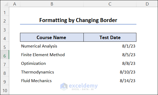
Changing Border:

Here in the image below, we can see there is no border in our dataset.

To add borders in this dataset select the dataset and from the Font group, click on Borders and select the suitable border. Here we chose All Borders.

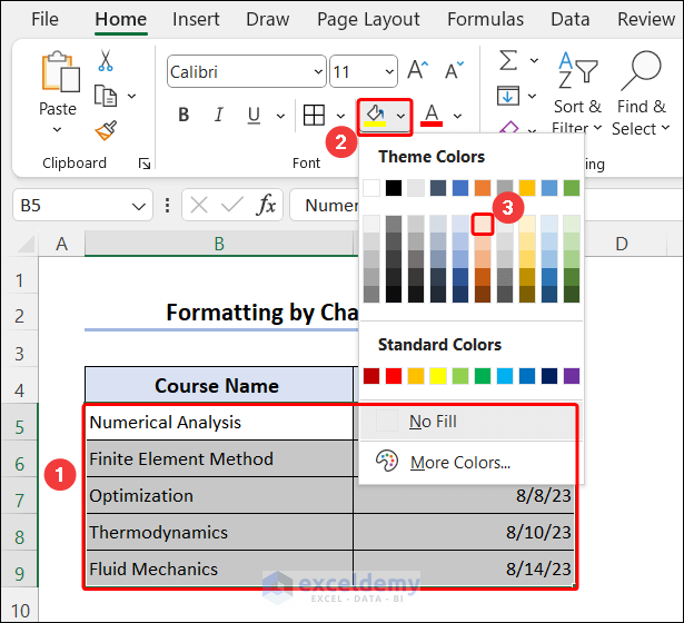
Fill Color Changing:

We can also change or add a fill color to the cells. To do this, first, select the dataset B5:C9. Then click on the Fill Color tool in the Font group from the dropdown menu we can choose our suitable fill color.

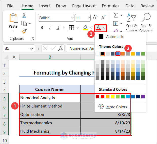
Changing Font Color:

We can also choose the font color from the Font group. Select the dataset, go to Font Color tool and from the dropdown select the font color. Here we have selected blue as our font color.

After applying all the changes the dataset will look like the image given below.

3.3. Working with Alignment Options to Change Cell Alignment

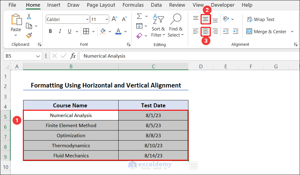
Changing Horizontal and Vertical Alignment:

We can change the text alignment in a cell using the Alignment group from the Home tab. Select the dataset, then go to the Alignment group and select the alignment suitable for you. Here we have selected Middle and Center alignment.

Changing Text Angle:

We can change the text angle using the Orientation tool from the Alignment group. Here we want to change the alignment of the test dates.
So select cells C5:C9. Then go to Orientation and select the angle. Here we have selected the Angle Counterclockwise option.

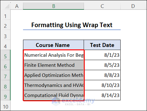
Wrapping Text in Cell:

If the text width is bigger than the cell width we will not see the full text in that cell. To make it visible either we have to increase the cell width or take the text to multiple lines. If we can’t increase the cell width, we can use the Wrap Text option.
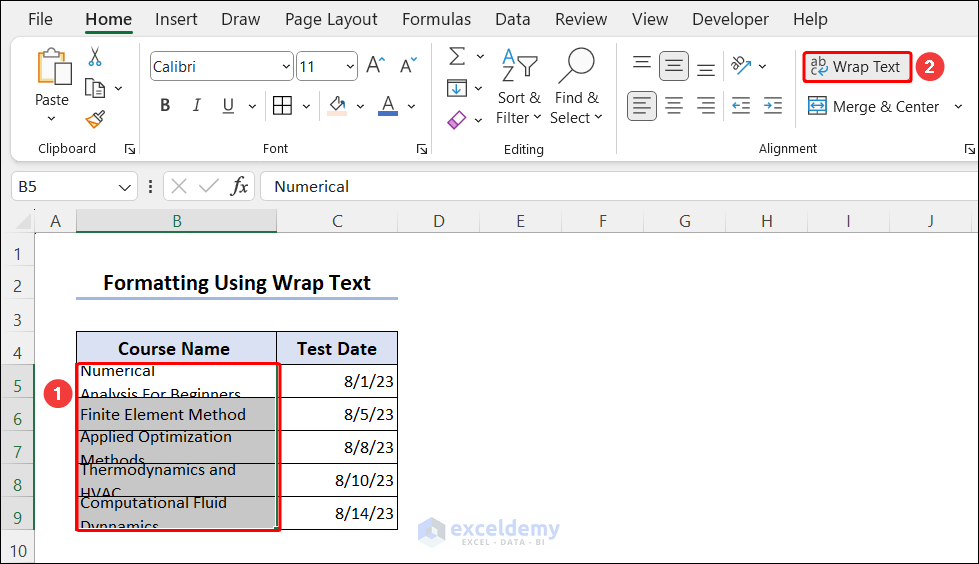
First, select the dataset. Here we have selected cells B5:B9.

Then select Wrap Text from the Alignment group. Now we can see the texts are in multiple lines. To make this visible we need to adjust the cell height.

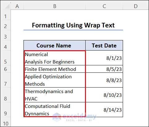
After adjusting the cell height we can now see the whole text without increasing the cell/column width.

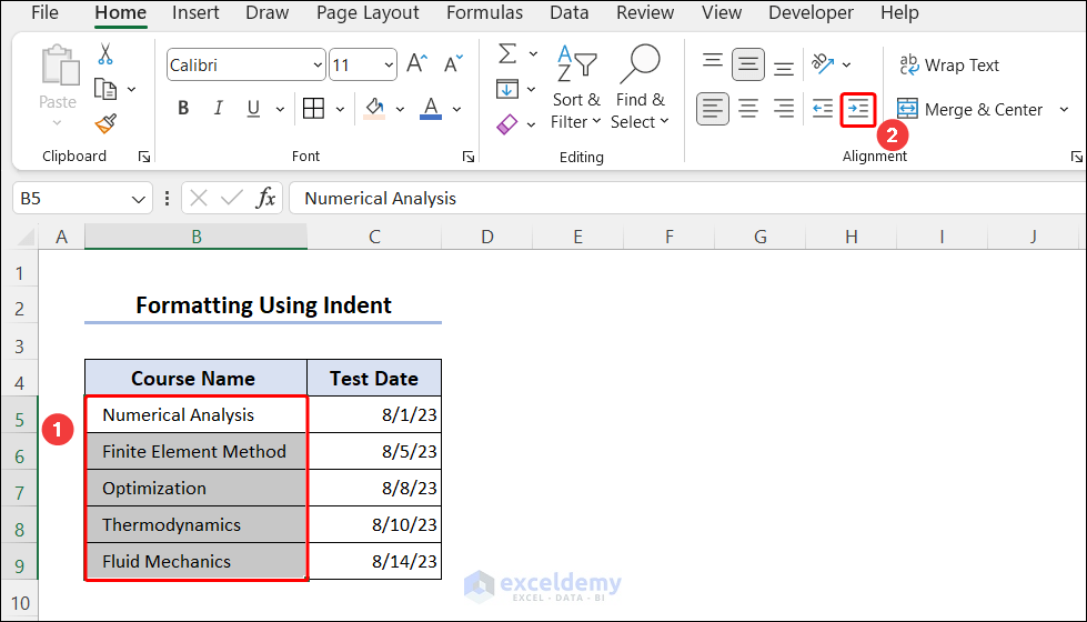
Indenting Text:

Sometimes we need to indent texts in a cell. We can also do this using the Alignment group.
Select the texts we want to indent. Then select Increase Indent.

Merge Cells:

We can also merge cells and make them one cell from the Excel Ribbon.

To do this select the cells we want to merge. Here we have selected B4 and C4 cells for merging. Then go to Merge & Center tool and from the dropdown select Merge & Center.

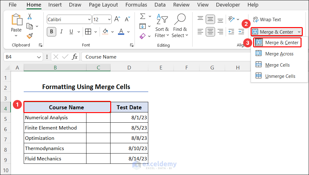
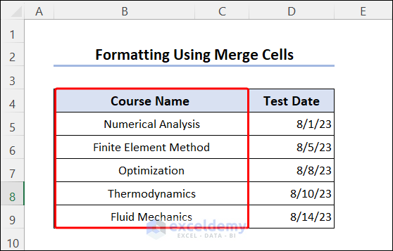
Now repeat the same process for the remaining cells in the B and C column.

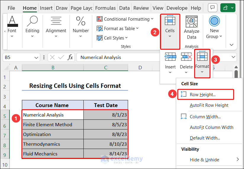
3.4. Resizing Columns and Rows

We can resize the row heights and column widths of the selected data range.
For this select the data range. Here we have selected cells B5:C9. Go to Cells >> Format >> Row Height. Then input the row height.

Enter the Row Height.

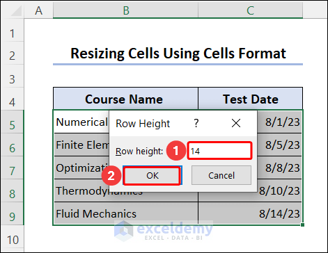
Here we can see the height of the selected cells has decreased.

We can also change the column width using the same process by selecting Column Width in the Format Option.

3.5. Applying Excel Styles with Cell Styles Group

We can also use some built-in cell styles to format the cell. There are many types of cell styles present in the Styles Group.
To use them, first, select the cells where you want to apply the style. Here we have selected cells B5:B9. Then from the Style group select Cell Styles. Then from the dropdown select any style for your use.

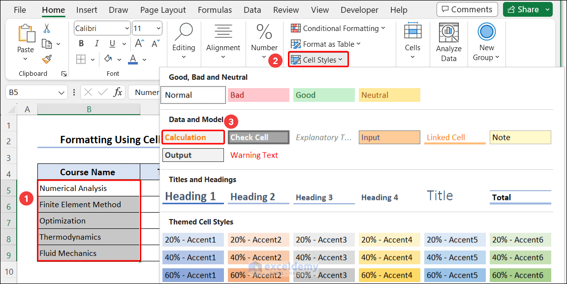
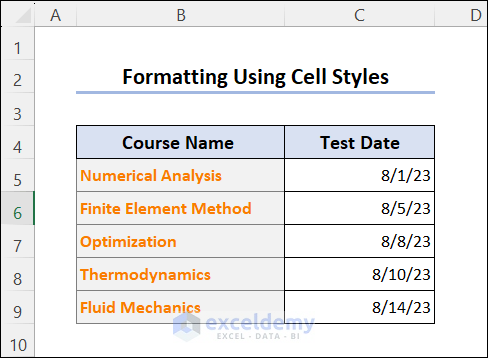
Here we have applied the Calculation style to the selected cells.

3.6. Using Number Format Dropdown to Change Data Type

We can change the number format from the Number group in the Home tab. In this article, we will change the date format to Long Date format.
Select the Test Date column and from the Number dropdown in the Home tab, select the Long Date format.

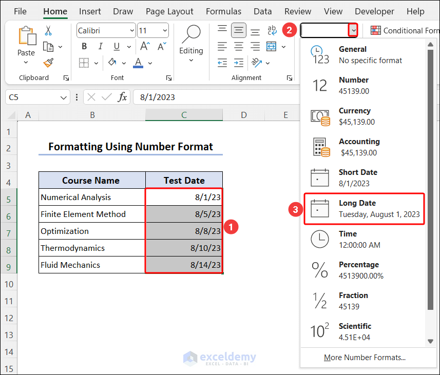
Now we can see the date format has been changed in the selected column.

3.7. Applying Conditional Formatting

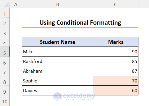
We can also change the cell format using Conditional Formatting. In this method, we will change the fill color of the cells that contain marks less than 85.
To do this select the Marks column and go to Conditional Formatting and select New Rule.

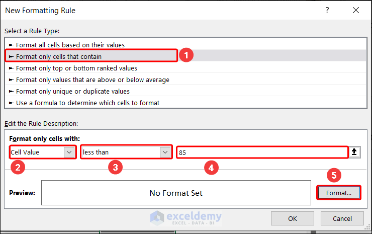
Then select “Format only cells that contain”. In the Edit the Rule Description, select Cell Value >> less than >> 85. Then select Format.

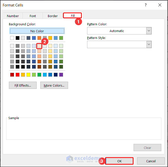
From the Format Cells window, go to the Fill tab and select the Background Color and click OK.

Now in the dataset, we can see all the cells that contain marks less than 85 have been highlighted.

4. Enabling and Using AutoFormat Tool

Enabling AutoFormat Tool

Now we will format the dataset using AutoFormat tool. But first, we need to enable the AutoFormat Tool.
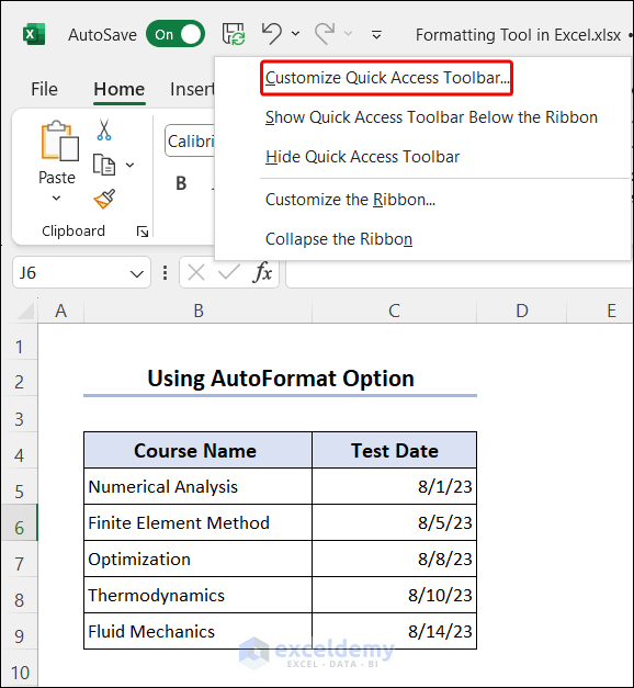
Take the cursor to the Quick Access Toolbar and right-click on it. From the options, select Customize Quick Access Toolbar.

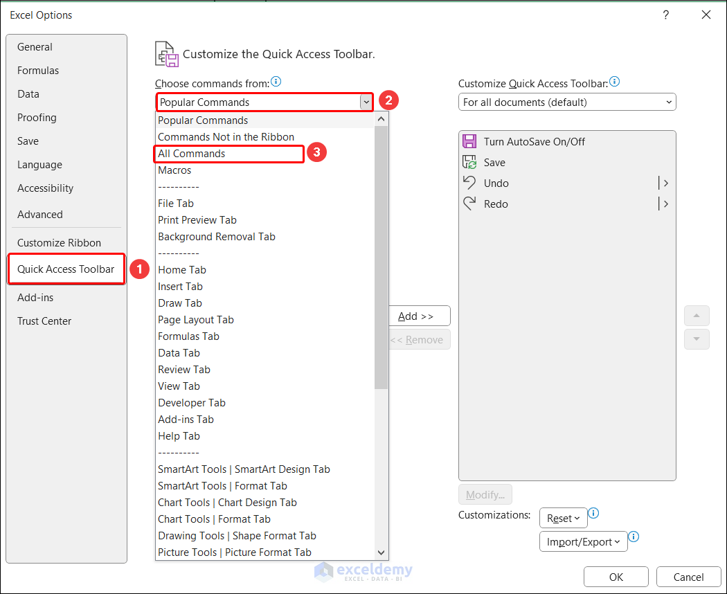
This will open the Excel Options dialog box. From there, go to the Quick Access Toolbar. From the Choose commands from dropdown, select All Commands.

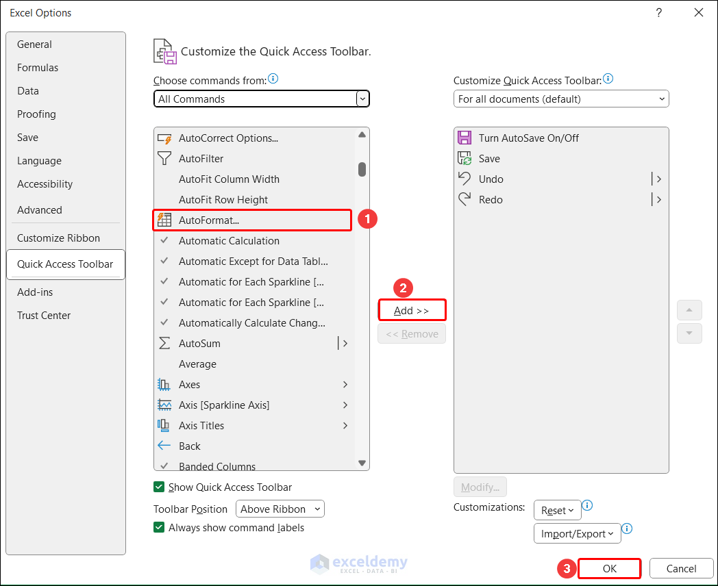
Then scroll down and select AutoFormat and click on Add. Click OK to close the dialog box.

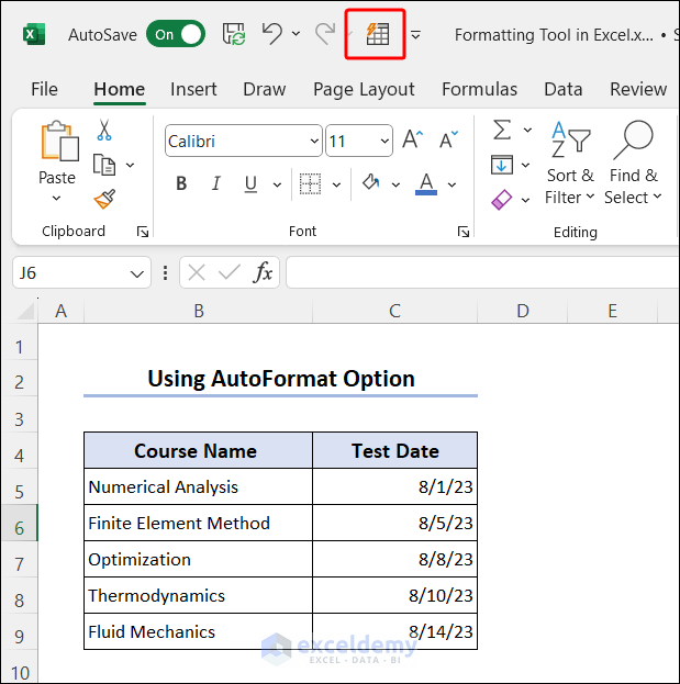
Now we can see the AutoFormat icon has been added in the Quick Access Toolbar.

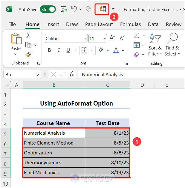
4.1 Using AutoFormat Option to Quickly Format Data

Now to apply AutoFormat, select the dataset and from the Quick Access Toolbar, click on AutoFormat.

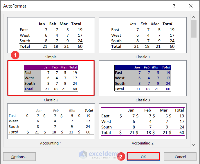
From the AutoFormat drop-down list select any format. Here we have selected Classic 2. Then click OK.

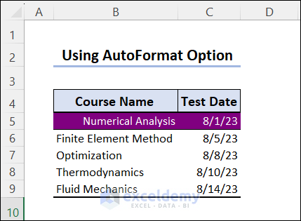
Now we can see our dataset format has changed according to the selected format from AutoFormat.

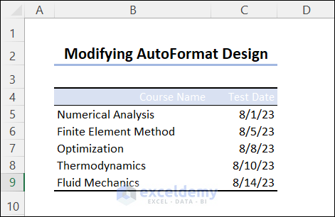
4.2 Modifying the Formatting Design in AutoFormat

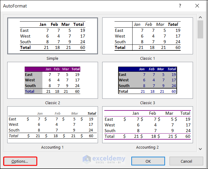
We can also modify the AutoFormat designs. Select the Dataset and click on AutoFormat.

Then Select Classic 2 and go to Options.

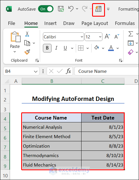
From AutoFormat window, remove the Patterns.

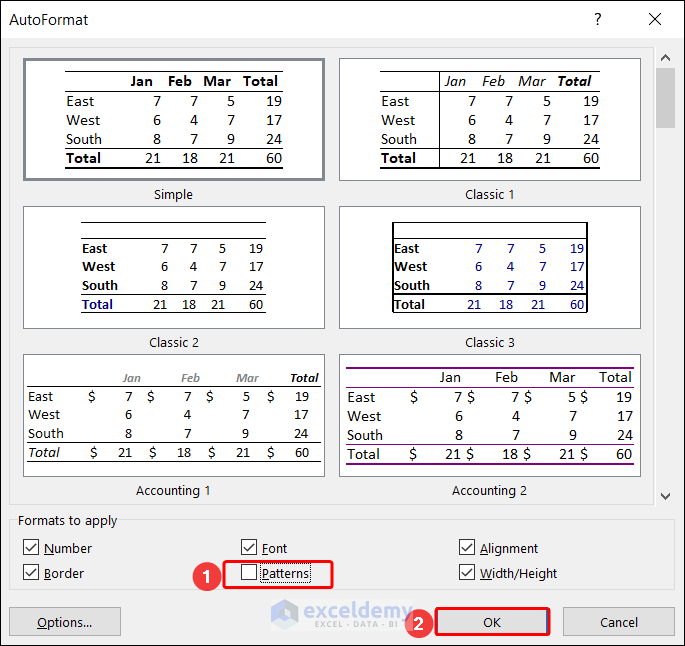
Now we can see the format is different from the previous one. So, using Options button, we can modify the auto formats.

5. Formatting Chart in Excel

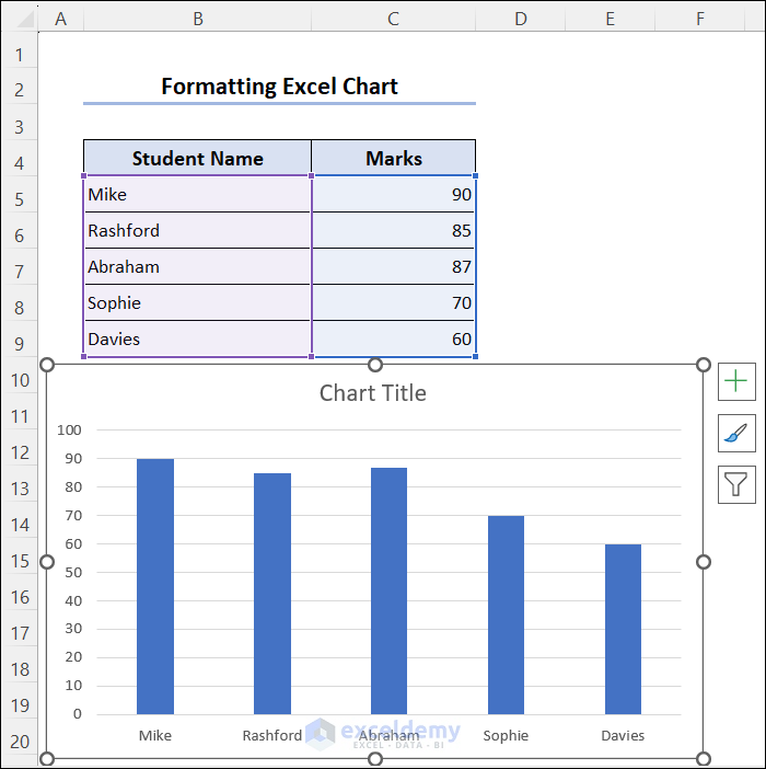
We can also format charts in Excel. But First, we need to insert a chart.
To insert a chart select the dataset then go to Insert >> Insert Column or Bar Chart >> 2D Column.

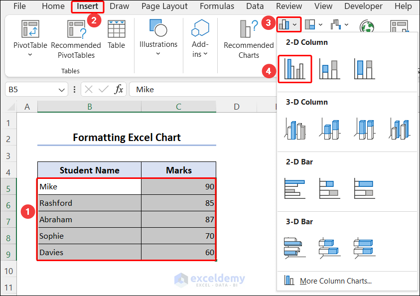
This will insert a bar chart based on the marks of the students.

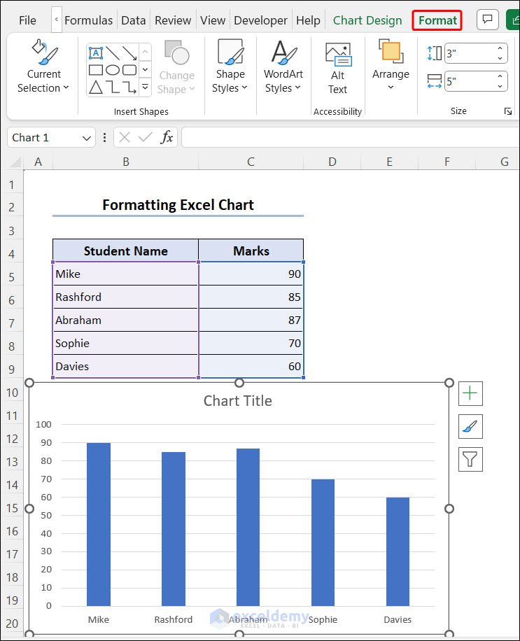
To format the chart select the chart and from the ribbon, go to the Format tab.

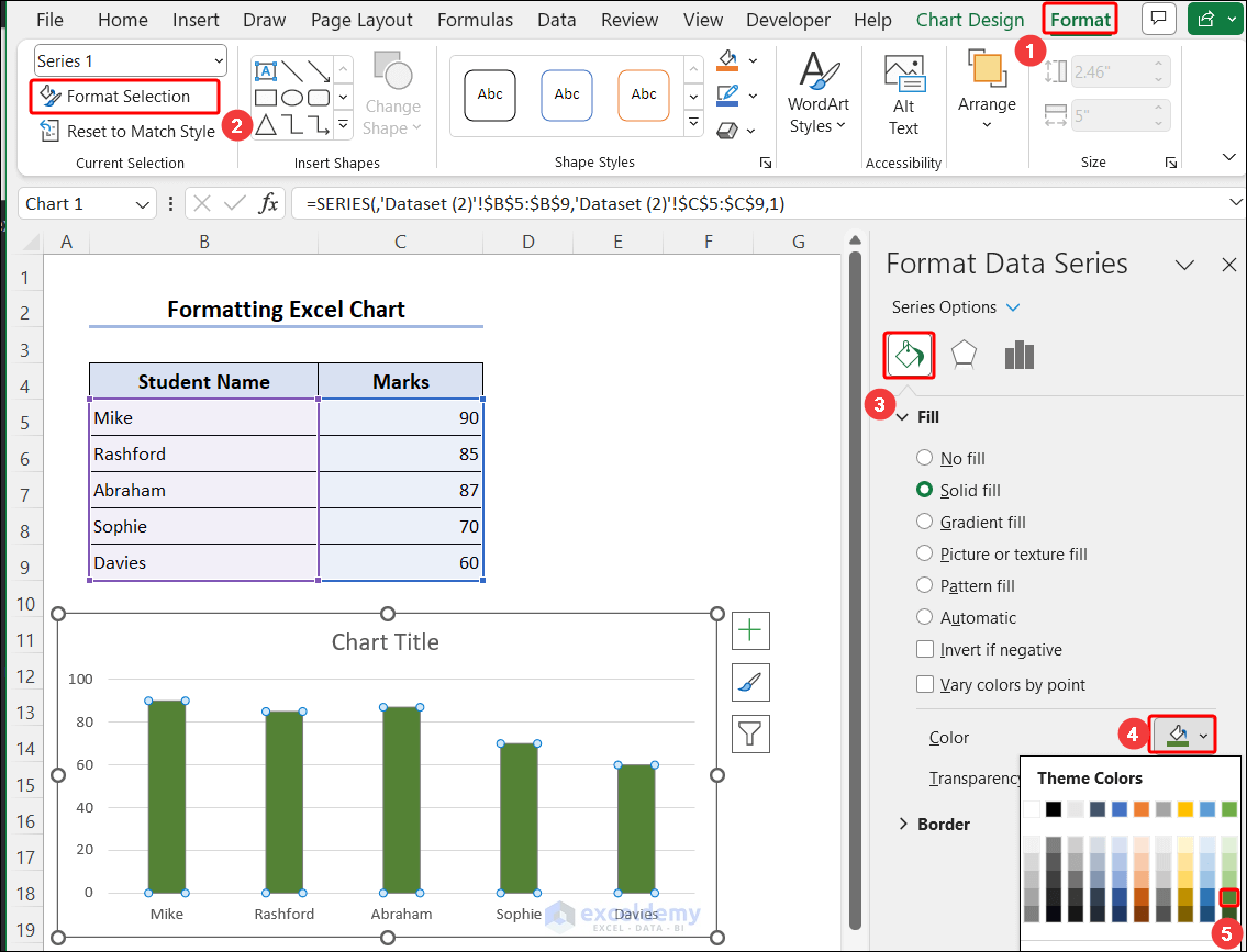
From the Format tab, select the Format Selection tool. The Format Data Series window will open.
From there, go to Fill Option. Here we can change the Color of the bars. We have selected a green color for the bars. Now we can see that the color of the bars has been changed to green.

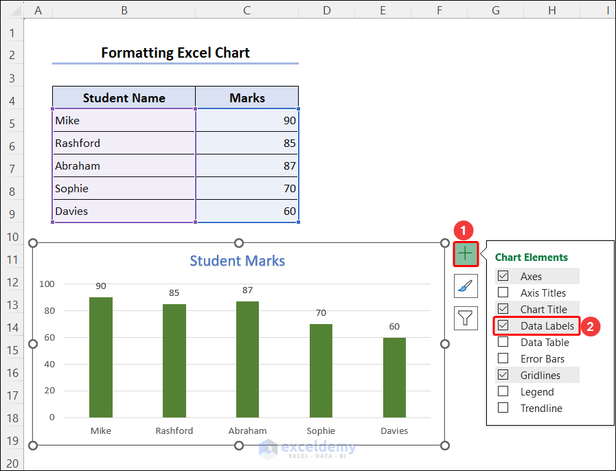
We can also give a title to the chart. In the Chart Title text box, enter the title for your chart. Here we named it Student Marks.
We can also change the font color of the chart title. For this select the text then go to Format and choose any WordArt Styles.

To add data labels select the chart click on the plus(+) icon and mark the Data Labels option. This will add data labels.

Frequently Asked Questions

1. What are the basic formatting tool in Excel?

You can do the basic formatting using the Format Cells dialog box. Here you can do all the basic formatting in Excel. Which includes Number Format, Font, Border, Fill, and Protection.

2. What are the common formatting features for Excel?

Some common formatting features are changing the Font, Font Color, Fill Color, Font Size, and Text Alignment. These are some common formatting we do regularly while using Microsoft Excel.

3. What is the purpose of formatting a worksheet in Excel?

Formatting helps to improve the readability of the worksheet. For example, highlighting the column heading will help us to easily identify what the column contains. Borders will also help us to identify the cells.

Conclusion

In this article, we tried to cover all the formatting tool for cells as well as Excel Charts. These formatting tools and methods will help you to learn the processes to apply these formats to your own dataset and make it easier to understand. We have also shown the effective uses of various formatting tools to format an Excel sheet quickly and easily. If you want to know more about the tips and tricks about Excel follow our website.

<< Go Back to Excel Cell Format | Learn Excel

Formatting Tool in Excel (Tool Types & Uses)