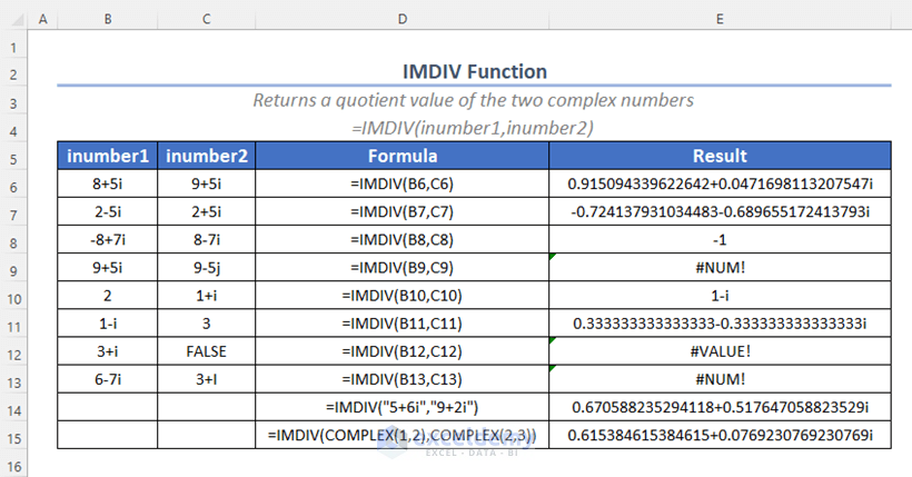
In Excel, we use the IMDIV function for calculating the quotient value after dividing a complex number by another complex number. In the following figure, we have demonstrated the usage of this function. So, let’s get into the main article.
IMDIV Function: Syntax & Arguments
⦿ Function Objective
The IMDIV function returns the result after dividing a complex number by another complex number.
⦿ Syntax
=IMDIV(inumber1, inumber2)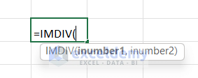
⦿ Arguments
| Argument | Required/Optional | Explanation |
|---|---|---|
| inumber1 | Required | The first complex number is the dividend. |
| inumber2 | Required | The second complex number is the divisor. |
⦿ Return Value
It returns the quotient value after dividing two complex numbers and the result will be in text format.
⦿ Version
The IMDIV function is available in Excel 2007 and later versions.
Excel IMDIV Function: 3 Examples
In the following examples, we demonstrated the usage of the IMDIV function in Excel. For creating this article, we have used the Microsoft Excel 365 version. However, you can use any other version at your convenience.
Example-1: Inserting Arguments Directly into IMDIV Function
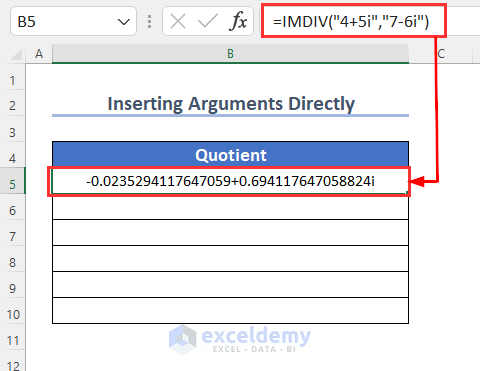
In this section, we will insert the arguments directly into the IMDIV function and get the quotient values in the following table.
Steps:
- Type the following formula in cell B5.
=IMDIV("4+5i", "7-6i")Here, “4+5i” is the first complex number which is the dividend, and “7-6i” is the second complex number which is the divisor.
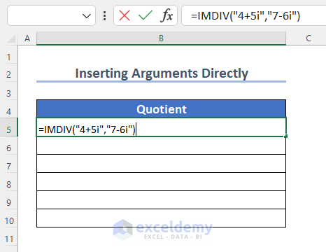
- Press ENTER.
As a result, we will get the following result after dividing two complex numbers.
Similarly, we used different complex numbers for the rest of the results.
Finally, we used the following formula to get the result in cell B10.
=IMDIV("1+5i","7+i")
Example-2: Using Cell Reference for IMDIV Function in Excel
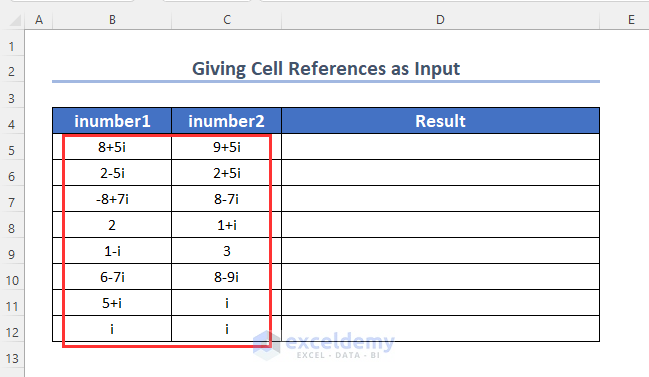
Here, we have two lists of complex numbers using which we will get the quotient value after dividing each complex number from one list by another complex number from the second list.
Steps:
- Type the following formula in cell D5 and press ENTER.
=IMDIV(B5, C5)Here, B5 is the first complex number which is the dividend, and C5 is the second complex number which is the divisor.
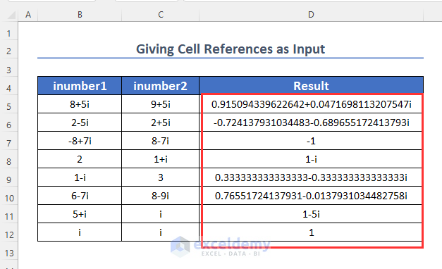
- Drag down the Fill Handle tool.

In this way, we get the results for the rest of the cells after dividing the complex numbers from column inumber1 by the complex numbers from column inumber2.
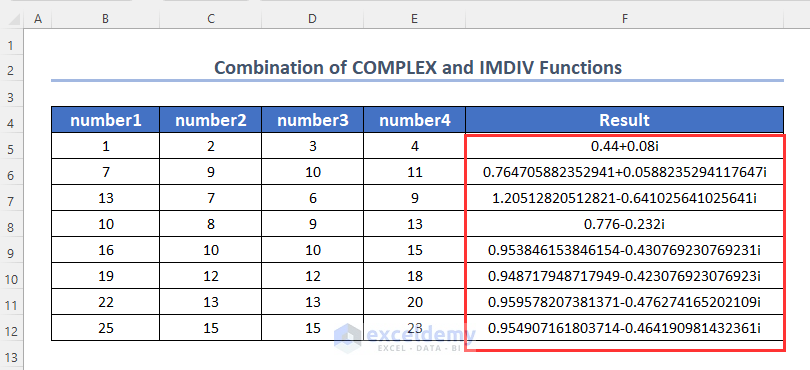
Example-3: Applying a Combination of COMPLEX and IMDIV Functions in Excel
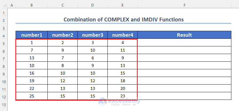
In the following table, we can see that we have 4 lists containing different real numbers. So, using these numbers and the COMPLEX function we will convert them into two complex numbers. Finally, the IMDIV function will give us the resultant value after dividing the first complex number by the second one.
Steps:
- Type the following formula in cell F5 and press ENTER.
=IMDIV(COMPLEX(B5, C5), COMPLEX(D5, E5))Formula Breakdown
- COMPLEX(B5, C5) → becomes
- COMPLEX(1, 2) → returns the complex number with a real number 1 and complex number 2.
- Output → 1+2i
- COMPLEX(1, 2) → returns the complex number with a real number 1 and complex number 2.
- COMPLEX(D5, E5) → becomes
- COMPLEX(3, 4) → returns the complex number with a real number 3 and complex number 4.
- Output → 3+4i
- COMPLEX(3, 4) → returns the complex number with a real number 3 and complex number 4.
- IMDIV(COMPLEX(B5, C5), COMPLEX(D5, E5)) → becomes
- IMDIV(“1+2i”, “3+4i”) → returns the quotient value
- Output → 0.44+0.08i
- IMDIV(“1+2i”, “3+4i”) → returns the quotient value
- Drag down the Fill Handle tool.

Finally, we will get the following resultant values.
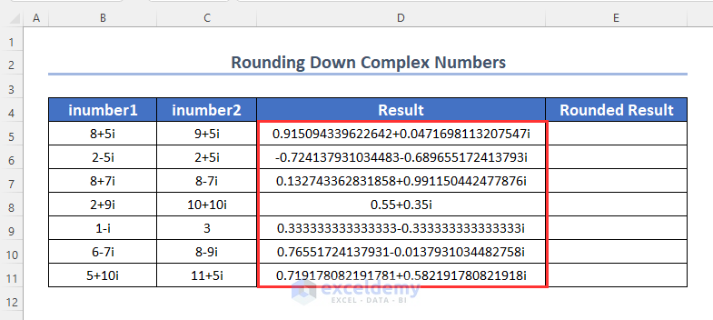
How to Round Down a Complex Number in Excel
After using the IMDIV function the resultant values become so large after the decimal point, so we need to round down this value to clearly understand it. But the complex numbers can not be rounded down easily. So, we need to use a specialized formula for this purpose.
Steps:
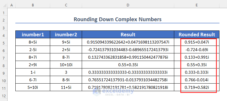
- Type the following formula in cell E5 and press ENTER.
=COMPLEX(VALUE(TEXT(IMREAL(D5), "0.000")), VALUE(TEXT(IMAGINARY(D5),"0.000")))Formula Breakdown
- IMREAL(D5) → becomes
- IMREAL(0.915094339622642+0.0471698113207547i) → The IMREAL function returns the real part of the complex number.
- Output → 0.915094339622642
- IMREAL(0.915094339622642+0.0471698113207547i) → The IMREAL function returns the real part of the complex number.
- TEXT(IMREAL(D5), “0.000”) → becomes
- TEXT(0.915094339622642, “0.000”) → The TEXT function will change the format of this number and round down it up to 3 decimal points.
- Output → “0.915”
- TEXT(0.915094339622642, “0.000”) → The TEXT function will change the format of this number and round down it up to 3 decimal points.
- VALUE(TEXT(IMREAL(D5), “0.000”)) → becomes
- VALUE(“0.915”) → The VALUE function will convert the text into a number.
- Output → 0.915
- VALUE(“0.915”) → The VALUE function will convert the text into a number.
- IMAGINARY(D5) → becomes
- IMAGINARY(0.915094339622642+0.0471698113207547i) → The IMAGINARY function will return the imaginary part of the complex number
- Output → 0.0471698113207547
- IMAGINARY(0.915094339622642+0.0471698113207547i) → The IMAGINARY function will return the imaginary part of the complex number
- TEXT(IMAGINARY(D5), “0.000”) → becomes
- TEXT(0.0471698113207547, “0.000”) → The TEXT function will change the format of this number and round down it up to 3 decimal points.
- Output → “0.047”
- TEXT(0.0471698113207547, “0.000”) → The TEXT function will change the format of this number and round down it up to 3 decimal points.
- VALUE(“0.047”) → The VALUE function will convert the text into a number.
- Output → 0.047
- COMPLEX(VALUE(TEXT(IMREAL(D5), “0.000”)), VALUE(TEXT(IMAGINARY(D5),”0.000″))) → becomes
- COMPLEX(0.915, 0.047) → returns the complex number with a real number 915 and complex number 0.047.
- Output → 0.915+0.047i
- COMPLEX(0.915, 0.047) → returns the complex number with a real number 915 and complex number 0.047.
- Drag down the Fill Handle tool.

Finally, we have reduced the numbers after the points from the following complex numbers.
Things to Remember
- You can not use 2 imaginary number indicators; i, and j, for indicating two complex numbers inside the IMDIV function. If you combine these indicators for two complex numbers then the function will return the #NUM! error.
- For indicating a complex number we have to use a lowercase i or j, not uppercase I or J.
- If you use any logical boolean value as an argument for the IMDIV function then you will get the #VALUE! error.
- The final note is that you can not put 0 as the second argument in the function.
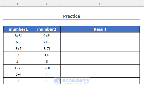
Practice Section
To practice by yourself, we have created a practice section on the right side of each sheet.
Download Practice Workbook
Conclusion
In this article, we have discussed different ways to use the IMDIV function in Excel. Hope these methods will help you a lot. If you have any further queries, then leave a comment below.
Related Article
- How to Use IMSUB Function in Excel
- How to Use Excel IMSUM Function
- How to Use IMPRODUCT Function in Excel
- How to Use Excel IMABS Function
<< Go Back to Excel Functions | Learn Excel

