Excel’s split screen option is a great way to view your work simultaneously at the same time. You can even visualize your work vertically or horizontally using this feature. In this article, we will show you how you can split screen in Excel.
Split Screen in Excel: 3 Ways
In this section, you will learn how to split the Excel screen into four sections, into two vertical sections and into two horizontal sections.
1. Splitting the Screen into Four Sections in Excel
The steps to split the screen in Excel are shown below.
Steps:
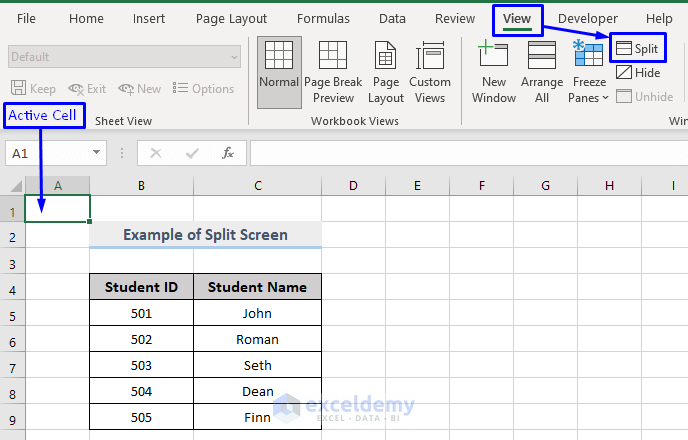
- First, you have to make sure that you keep cell A1 as your active cell.
- Then in the ribbon, go to tab View -> Split in the Windows group.
- If you click the Split. Then you will see your screen is now divided into four sections by both horizontal and vertical lines that appeared in the middle of the worksheet.
- Each of the four quadrants created should be a copy of the original sheet.
- There should be also two horizontal and vertical scroll bars appearing at the bottom and on the right side of the screen.

- You can use the drag bars from each quadrant of the worksheet to reposition the screen.
2. Dividing Excel Screen into Two Sections Vertically
The Split option in Excel lets you divide the screen into four sections. But what if you want to separate the screen into two sections?
Steps to divide the Excel screen into two vertical sections are given below.
Steps:
- When you have your screen split into four panes, you can use the horizontal line or the split bar from the right side to drag the whole horizontal section out of the screen.
For example, to have the screen split vertically, drag the horizontal line or the split bar from the right side of the screen to the far bottom or top of the worksheet, leaving only the vertical bar on the screen.
Notice the gif below to understand more.

3. Splitting the Screen into Two Sections Horizontally
In the same way, shown above, you can also separate the screen into two horizontal sections.
Steps:
- When you have your screen split into four panes, you can use the vertical line or the split bar from the bottom side to drag the whole vertical section out of the screen.
For instance, to have the screen split horizontally, drag the vertical line or the split bar from the bottom side of the screen to the far left or right of the worksheet, leaving only the horizontal bar on the screen.
See the gif below to understand more.

Removing Split Screen
To remove the split-screen all you have to do is,
- Click on the View -> Split. It will turn off the split-screen feature and your screen will consist of only one worksheet.
Or,
- Drag both the split bars to the edges of the screen, it will also turn the split-screen icon off from the ribbon and you will have only one screen to work in Excel.
Download Workbook
You can download the free practice Excel workbook from here.
Conclusion
This article showed you how to split the screen in Excel in 3 different ways. I hope this article has been very beneficial to you. Feel free to ask if you have any questions regarding the topic.
Related Articles
- How to Split Excel Sheet into Multiple Worksheets
- How to Split Sheet into Multiple Sheets Based on Rows in Excel
- How to Split Excel Sheet into Multiple Sheets Based on Column Value
- How to Split Excel Sheet into Multiple Files
- How to Enable Side-by-Side View with Vertical Alignments in Excel
- How to View Excel Sheets in Separate Windows
- [Fix:] Excel View Side by Side Not Working
- Excel VBA: Split Sheet into Multiple Sheets Based on Rows
- How to Split a Workbook to Separate Excel Files with VBA Code
<< Go Back to Split Excel Cell | Excel Worksheets | Learn Excel

