Despite having the same type of information for various occasions in different worksheets, we can consolidate them in a single worksheet. It will combine information from multiple worksheets into one. To fulfill this purpose, there is a command named Consolidate in Excel. In this article, I am going to show you how to consolidate information in Excel in two simple ways.
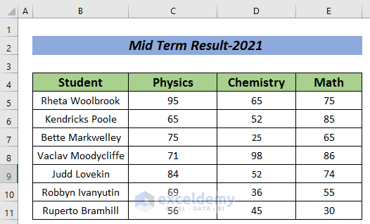
For more clarification, I am going to use two datasets. Dataset-1 contains the Mid-Term Result- 2021 of a student in Physics, Chemistry, and Math.
Similarly, Dataset-2 contains the Annual Result- 2021 of a student in Physics, Chemistry, and Math.

We will try to consolidate these results and make a consolidated one.
How to Consolidate Information in Excel: 2 Simple Ways
1. Consolidate Information with Excel Consolidate Feature
The best and simplest way to consolidate data from multiple ranges in Excel is to use the Consolidate feature in Excel. We can do it easily just by following the steps mentioned below.
Steps:
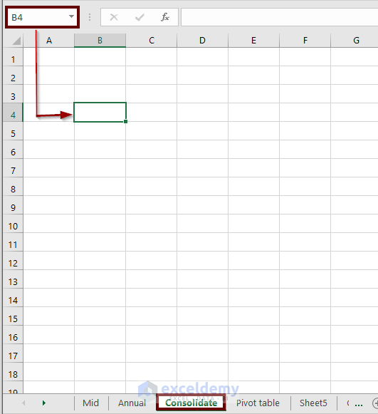
- First, create a new worksheet. Here, I created a new worksheet and named it.
- Next, pick a cell for the consolidation (i.e. B4).
- Now, go to the Data tab.
- Click on the Consolidate feature from the ribbon.

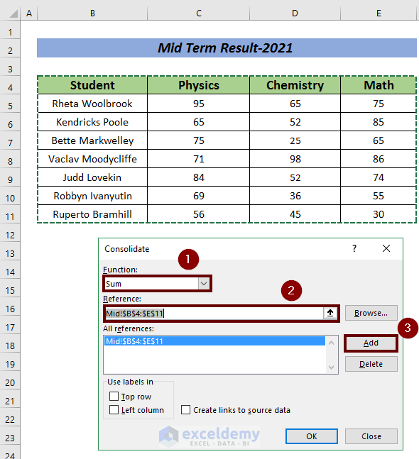
A Consolidate wizard will appear.
- Pick a function according to your need (i.e. SUM).
- Select the range of the particular worksheet in the Reference section (i.e. B4:E11 cells in the Mid worksheet).
- Next, click on Add.
- After that, select the information range of another worksheet in the Reference section (i.e. B4:E11 cells in the Annual worksheet).
- Press on Add.
- Now, check all the boxes.
- Finally, press OK to finish the process.

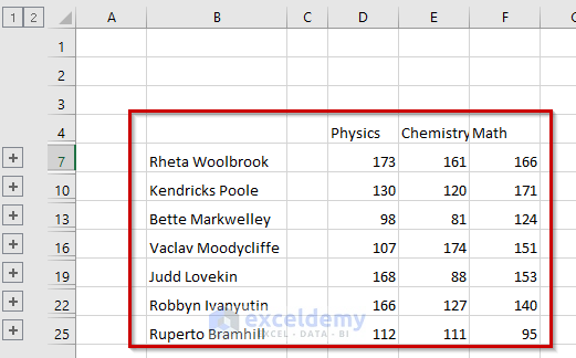
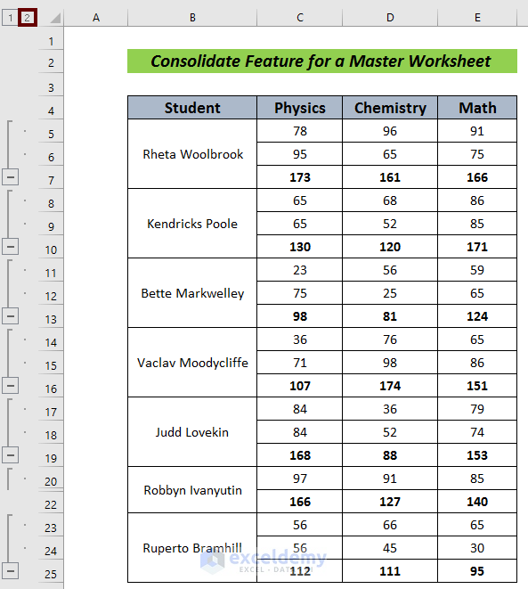
We will have our consolidated information on the master worksheet.
You can decorate your consolidated information according to your choice.
There will be two buttons named 1 and 2 which will control the consolidated information’s view. Button 1 shows the consolidated final information hiding all the data collected from the multiple worksheets.

On the other hand, button 2 shows all the information keeping the same type of information in groups.
2. Using Pivot Table to Consolidate Information
Pivot Table is another way to consolidate information in Excel. This process is mainly used to organize the disorganized information of a dataset.
To explain the whole consolidation process using the Pivot Table, I am going to use a new dataset about the salary structure of a company. I explained the salary structure of that company using the Name, Department, and Salary columns.
Steps:
- First, select all the cells that you want to consolidate(i.e. B4:D14).
- Secondly, go to the Insert tab.
- Next, click on the Pivot Table option from the ribbon.

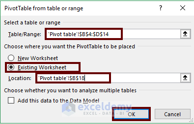
The Table/Range section will be automatically filled as I have mentioned the range in the first step.
- Choose an option where you want to have your Pivot Table. I decided to have the Pivot Table in the Existing Worksheet.
- If you select the Existing Worksheet, select the cell where you want to have the table in the Location section(i.e. B18).
- Then, press OK.
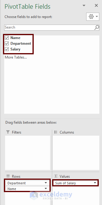
We will be able to see the Pivot Table format in the selected cell. A Pivot Table Fields box will appear on the right side of the worksheet.

- Mention the Rows and Values from the Pivot Table Fields I have selected Department and Name as the Rows where Department is the primary label. I have also selected Salary as Values.
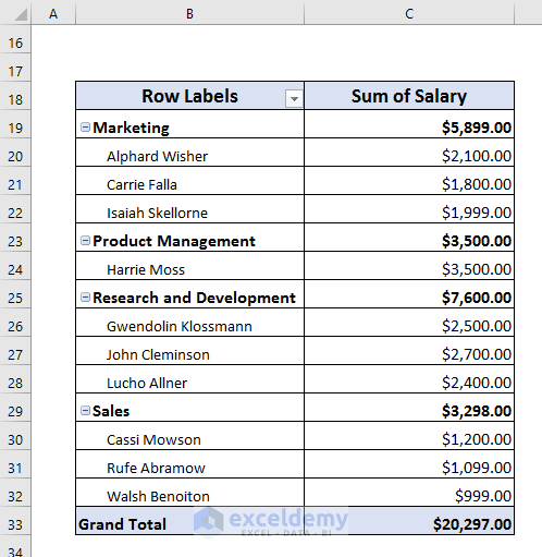
After that, we will have our consolidated data on the selected location.

You can modify your data if you wish to do so.
Download Practice Workbook
Conclusion
I have tried to simply explain the two simple ways to consolidate information in Excel. It will be a matter of great pleasure for me if this article could help any Excel user even a little. For any further queries, comment below.
<< Go Back To Consolidation in Excel | Merge Sheets in Excel | Merge in Excel | Learn Excel

